
User`s guide
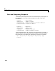
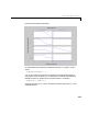

Table Of Contents
- Preface
- Quick Start
- LTI Models
- Introduction
- Creating LTI Models
- LTI Properties
- Model Conversion
- Time Delays
- Simulink Block for LTI Systems
- References
- Operations on LTI Models
- Arrays of LTI Models
- Model Analysis Tools
- The LTI Viewer
- Introduction
- Getting Started Using the LTI Viewer: An Example
- The LTI Viewer Menus
- The Right-Click Menus
- The LTI Viewer Tools Menu
- Simulink LTI Viewer
- Control Design Tools
- The Root Locus Design GUI
- Introduction
- A Servomechanism Example
- Controller Design Using the Root Locus Design GUI
- Additional Root Locus Design GUI Features
- References
- Design Case Studies
- Reliable Computations
- Reference
- Category Tables
- acker
- append
- augstate
- balreal
- bode
- c2d
- canon
- care
- chgunits
- connect
- covar
- ctrb
- ctrbf
- d2c
- d2d
- damp
- dare
- dcgain
- delay2z
- dlqr
- dlyap
- drmodel, drss
- dsort
- dss
- dssdata
- esort
- estim
- evalfr
- feedback
- filt
- frd
- frdata
- freqresp
- gensig
- get
- gram
- hasdelay
- impulse
- initial
- inv
- isct, isdt
- isempty
- isproper
- issiso
- kalman
- kalmd
- lft
- lqgreg
- lqr
- lqrd
- lqry
- lsim
- ltiview
- lyap
- margin
- minreal
- modred
- ndims
- ngrid
- nichols
- norm
- nyquist
- obsv
- obsvf
- ord2
- pade
- parallel
- place
- pole
- pzmap
- reg
- reshape
- rlocfind
- rlocus
- rltool
- rmodel, rss
- series
- set
- sgrid
- sigma
- size
- sminreal
- ss
- ss2ss
- ssbal
- ssdata
- stack
- step
- tf
- tfdata
- totaldelay
- zero
- zgrid
- zpk
- zpkdata
- Index

1 Quick Start
1-20
Control Design Tools
The Control System Toolbox supports three mainstream control design
methodologies: gain selection from root locus, pole placement, and
linear-quadratic-Gaussian (LQG) regulation. The first two techniques are
covered by the
rlocus and place commands. The LQG design tools include
commands to compute the LQ-optimal state-feedback gain (
lqr, dlqr,and
lqry), to design the Kalman filter (kalman), and to form the resulting LQG
regulator (
lqgreg). See “LQG Design” on page 7-8 for more information.
As an example of LQG design, consider the regulation problem illustrated by
Figure 1-1. The goal is to regulate the plant output around zero. The system
is driven by the white noise disturbance , there is some measurement noise
, and the noise intensities are given by
The cost function
is used to specify the trade-off between regulation performance and cost of
control. Note that an open-loop state-space model is
where is a state-space realization of .
y
d
n
Ed
2
() 1,= En
2
() 0.01=
Ju() 10y
2
u
2
+()td
0
∞
∫
=
x
·
Ax Bu Bd++= (state equations)
y
n
Cx n+= (measurements)
ABC
,,() 100 s
2
s 100++()⁄