
User`s guide
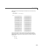
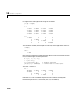

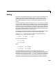
Table Of Contents
- Preface
- Quick Start
- LTI Models
- Introduction
- Creating LTI Models
- LTI Properties
- Model Conversion
- Time Delays
- Simulink Block for LTI Systems
- References
- Operations on LTI Models
- Arrays of LTI Models
- Model Analysis Tools
- The LTI Viewer
- Introduction
- Getting Started Using the LTI Viewer: An Example
- The LTI Viewer Menus
- The Right-Click Menus
- The LTI Viewer Tools Menu
- Simulink LTI Viewer
- Control Design Tools
- The Root Locus Design GUI
- Introduction
- A Servomechanism Example
- Controller Design Using the Root Locus Design GUI
- Additional Root Locus Design GUI Features
- References
- Design Case Studies
- Reliable Computations
- Reference
- Category Tables
- acker
- append
- augstate
- balreal
- bode
- c2d
- canon
- care
- chgunits
- connect
- covar
- ctrb
- ctrbf
- d2c
- d2d
- damp
- dare
- dcgain
- delay2z
- dlqr
- dlyap
- drmodel, drss
- dsort
- dss
- dssdata
- esort
- estim
- evalfr
- feedback
- filt
- frd
- frdata
- freqresp
- gensig
- get
- gram
- hasdelay
- impulse
- initial
- inv
- isct, isdt
- isempty
- isproper
- issiso
- kalman
- kalmd
- lft
- lqgreg
- lqr
- lqrd
- lqry
- lsim
- ltiview
- lyap
- margin
- minreal
- modred
- ndims
- ngrid
- nichols
- norm
- nyquist
- obsv
- obsvf
- ord2
- pade
- parallel
- place
- pole
- pzmap
- reg
- reshape
- rlocfind
- rlocus
- rltool
- rmodel, rss
- series
- set
- sgrid
- sigma
- size
- sminreal
- ss
- ss2ss
- ssbal
- ssdata
- stack
- step
- tf
- tfdata
- totaldelay
- zero
- zgrid
- zpk
- zpkdata
- Index

Choice of LTI Model
10-13
Note also that the eigenvectors have changed.
[vc,dc] = eig(Ac)
vc =
–0.5017 0.2353 0.0510 0.0109
–0.8026 0.7531 0.4077 0.1741
–0.3211 0.6025 0.8154 0.6963
–0.0321 0.1205 0.4077 0.6963
dc =
10.0000 0 0 0
0 5.0000 0 0
0 0 2.0000 0
0 0 0 1.0000
The condition number of the new eigenvector matrix
cond(vc)
ans =
34.5825
is thirty time s larg er.
Thephenomenon illustrated aboveis not unusual. Matricesin companion form
or control labl e/obs erva ble canonical form (lik e
Ac) typicall y have
worse-conditioned eigensystems than matrices in general state-space form
(like
A). This me ans t hat their ei genv alues and eigenve ctor s are more se nsi tive
topert urbatio n.The problem genera llyg etsf arw or se forhigher-ord ers ystems .
Working with high-order transfer function mo dels and conv erting the m bac k
and forth to state space is numerically risky.
In summary, the main numerical problems t o be aware of in dealing with
transfer function m odels (and hence, calcula tions involving po lynomia ls) are:
• The potentially large range of numbers leads to ill -conditioned problems,
especial ly w hen s uch mod els are link ed t oge ther gi ving hig h-ord er
polynomials.