
User`s guide
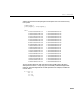
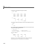

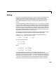
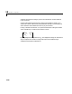
Table Of Contents
- Preface
- Quick Start
- LTI Models
- Introduction
- Creating LTI Models
- LTI Properties
- Model Conversion
- Time Delays
- Simulink Block for LTI Systems
- References
- Operations on LTI Models
- Arrays of LTI Models
- Model Analysis Tools
- The LTI Viewer
- Introduction
- Getting Started Using the LTI Viewer: An Example
- The LTI Viewer Menus
- The Right-Click Menus
- The LTI Viewer Tools Menu
- Simulink LTI Viewer
- Control Design Tools
- The Root Locus Design GUI
- Introduction
- A Servomechanism Example
- Controller Design Using the Root Locus Design GUI
- Additional Root Locus Design GUI Features
- References
- Design Case Studies
- Reliable Computations
- Reference
- Category Tables
- acker
- append
- augstate
- balreal
- bode
- c2d
- canon
- care
- chgunits
- connect
- covar
- ctrb
- ctrbf
- d2c
- d2d
- damp
- dare
- dcgain
- delay2z
- dlqr
- dlyap
- drmodel, drss
- dsort
- dss
- dssdata
- esort
- estim
- evalfr
- feedback
- filt
- frd
- frdata
- freqresp
- gensig
- get
- gram
- hasdelay
- impulse
- initial
- inv
- isct, isdt
- isempty
- isproper
- issiso
- kalman
- kalmd
- lft
- lqgreg
- lqr
- lqrd
- lqry
- lsim
- ltiview
- lyap
- margin
- minreal
- modred
- ndims
- ngrid
- nichols
- norm
- nyquist
- obsv
- obsvf
- ord2
- pade
- parallel
- place
- pole
- pzmap
- reg
- reshape
- rlocfind
- rlocus
- rltool
- rmodel, rss
- series
- set
- sgrid
- sigma
- size
- sminreal
- ss
- ss2ss
- ssbal
- ssdata
- stack
- step
- tf
- tfdata
- totaldelay
- zero
- zgrid
- zpk
- zpkdata
- Index

Choice of LTI Model
10-11
and the conversionfrom zero-pole-gainto state s pace incurs no loss of accuracy
in the poles.
format long e
[sort(eig(a1)) sort(eig(a2))]
ans =
9.999999999998792e-01 1.000000000000000e+00
2.000000000001984e+00 2.000000000000000e+00
3.000000000475623e+00 3.000000000000000e+00
3.999999981263996e+00 4.000000000000000e+00
5.000000270433721e+00 5.000000000000000e+00
5.999998194359617e+00 6.000000000000000e+00
7.000004542844700e+00 7.000000000000000e+00
8.000013753274901e+00 8.000000000000000e+00
8.999848908317270e+00 9.000000000000000e+00
1.000059459550623e+01 1.000000000000000e+01
1.099854678336595e+01 1.100000000000000e+01
1.200255822210095e+01 1.200000000000000e+01
1.299647702454549e+01 1.300000000000000e+01
1.400406940833612e+01 1.400000000000000e+01
1.499604787386921e+01 1.500000000000000e+01
1.600304396718421e+01 1.600000000000000e+01
1.699828695210055e+01 1.700000000000000e+01
1.800062935148728e+01 1.800000000000000e+01
1.899986934359322e+01 1.900000000000000e+01
2.000001082693916e+01 2.000000000000000e+01
There is another difficulty with transfer function models when real ized in
state-space form with
ss. They may give rise to badly conditioned eigenvector
matrices, even if the eigenvalues are well separated. For example, consider the
normal matrix
A = [5 4 1 1
4 5 1 1
1 1 4 2
1 1 2 4]