
User`s guide
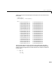

Table Of Contents
- Preface
- Quick Start
- LTI Models
- Introduction
- Creating LTI Models
- LTI Properties
- Model Conversion
- Time Delays
- Simulink Block for LTI Systems
- References
- Operations on LTI Models
- Arrays of LTI Models
- Model Analysis Tools
- The LTI Viewer
- Introduction
- Getting Started Using the LTI Viewer: An Example
- The LTI Viewer Menus
- The Right-Click Menus
- The LTI Viewer Tools Menu
- Simulink LTI Viewer
- Control Design Tools
- The Root Locus Design GUI
- Introduction
- A Servomechanism Example
- Controller Design Using the Root Locus Design GUI
- Additional Root Locus Design GUI Features
- References
- Design Case Studies
- Reliable Computations
- Reference
- Category Tables
- acker
- append
- augstate
- balreal
- bode
- c2d
- canon
- care
- chgunits
- connect
- covar
- ctrb
- ctrbf
- d2c
- d2d
- damp
- dare
- dcgain
- delay2z
- dlqr
- dlyap
- drmodel, drss
- dsort
- dss
- dssdata
- esort
- estim
- evalfr
- feedback
- filt
- frd
- frdata
- freqresp
- gensig
- get
- gram
- hasdelay
- impulse
- initial
- inv
- isct, isdt
- isempty
- isproper
- issiso
- kalman
- kalmd
- lft
- lqgreg
- lqr
- lqrd
- lqry
- lsim
- ltiview
- lyap
- margin
- minreal
- modred
- ndims
- ngrid
- nichols
- norm
- nyquist
- obsv
- obsvf
- ord2
- pade
- parallel
- place
- pole
- pzmap
- reg
- reshape
- rlocfind
- rlocus
- rltool
- rmodel, rss
- series
- set
- sgrid
- sigma
- size
- sminreal
- ss
- ss2ss
- ssbal
- ssdata
- stack
- step
- tf
- tfdata
- totaldelay
- zero
- zgrid
- zpk
- zpkdata
- Index

10 Reliable Computations
10-10
verylittle. Thisis true in general.Different roots have different sensitivitiesto
different perturbations. Computed roots may then be quite meaningless for a
polynomial, particularly high-order, with imprecisely known coefficients.
Finding all the roots of a polynomial (equivalently, the poles of a transfer
function or the eigenvalues of a matrix in controllable or observable canonical
form) is often an intrinsically sensitive problem. For a clear and detailed
treatment of the subject, including the tricky numerical problem o f deflation,
consult [6].
It is therefore preferable to work with the factored form of polynomials when
available. To compute a state-space model of the transfer function
defined above, for example, you could expand the denominator of , convert
the transfer function model to state space, and extract the state-space data by
H1 = tf(1,poly(1:20))
H1ss = ss(H1)
[a1,b1,c1] = ssdata(H1)
However, you should rather keep the denominator in fact ored form and work
with the zero-pole-gain representation of .
H2 = zpk([],1:20,1)
H2ss = ss(H2)
[a2,b2,c2] = ssdata(H2)
Indeed, the resulting state matrix a2 is better conditioned.
[cond(a1) cond(a2)]
ans =
2.7681e+03 8.8753e+01
Hs
()
H
Hs
()