
User`s guide
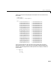


Table Of Contents
- Preface
- Quick Start
- LTI Models
- Introduction
- Creating LTI Models
- LTI Properties
- Model Conversion
- Time Delays
- Simulink Block for LTI Systems
- References
- Operations on LTI Models
- Arrays of LTI Models
- Model Analysis Tools
- The LTI Viewer
- Introduction
- Getting Started Using the LTI Viewer: An Example
- The LTI Viewer Menus
- The Right-Click Menus
- The LTI Viewer Tools Menu
- Simulink LTI Viewer
- Control Design Tools
- The Root Locus Design GUI
- Introduction
- A Servomechanism Example
- Controller Design Using the Root Locus Design GUI
- Additional Root Locus Design GUI Features
- References
- Design Case Studies
- Reliable Computations
- Reference
- Category Tables
- acker
- append
- augstate
- balreal
- bode
- c2d
- canon
- care
- chgunits
- connect
- covar
- ctrb
- ctrbf
- d2c
- d2d
- damp
- dare
- dcgain
- delay2z
- dlqr
- dlyap
- drmodel, drss
- dsort
- dss
- dssdata
- esort
- estim
- evalfr
- feedback
- filt
- frd
- frdata
- freqresp
- gensig
- get
- gram
- hasdelay
- impulse
- initial
- inv
- isct, isdt
- isempty
- isproper
- issiso
- kalman
- kalmd
- lft
- lqgreg
- lqr
- lqrd
- lqry
- lsim
- ltiview
- lyap
- margin
- minreal
- modred
- ndims
- ngrid
- nichols
- norm
- nyquist
- obsv
- obsvf
- ord2
- pade
- parallel
- place
- pole
- pzmap
- reg
- reshape
- rlocfind
- rlocus
- rltool
- rmodel, rss
- series
- set
- sgrid
- sigma
- size
- sminreal
- ss
- ss2ss
- ssbal
- ssdata
- stack
- step
- tf
- tfdata
- totaldelay
- zero
- zgrid
- zpk
- zpkdata
- Index

Choice of LTI Model
10-9
A major difficulty is the extreme sensitivity of the roots of a polynomial to its
coefficients. This example is adapted from Wilkinson, [6] as an illustration.
Consider the transfer function
The matrix of the companion realization of is
Despite the benign looking poles of the system (at –1,–2,..., –20) you are faced
with a rather large range in the elements of , from 1 to . But
the difficulties don’t stop here. Suppose the coefficient of in the transfer
function (or ) is perturbed from 210 to ( ).
Then, computed on a VAX (IEEE arithmetic has enough mantissa for o nly
), the poles of the perturbed transfer function (equivalently, the
eigenvalues of ) are
eig(A)'
ans =
Columns 1 through 7
–19.9998 –19.0019 –17.9916 –17.0217 –15.9594 –15.0516 –13.9504
Columns 8 through 14
–13.0369 –11.9805 –11.0081 –9.9976 –9.0005 –7.9999 –7.0000
Columns 15 through 20
–6.0000 –5.0000 –4.0000 –3.0000 –2.0000 –1.0000
The problem here is not roundoff. Rather, high-order polynomials are simply
intrinsically very sensitive, even when the zeros are well separated. In this
case, a relative perturbation of the order of induced relative
perturbations of the order of in someroots. But someof the roots changed
Hs()
1
s 1+()s2+()... s 20+()
-------------------------------------------------------------
1
s
20
210s
19
... 20!+++
-----------------------------------------------------------==
A
Hs
()
A
010...0
001...0
::..:
00....1
20!– .....210–
=
A
20! 2.4 10
18
×≈
s
19
Ann
,() 210 2
23
–
+ 2
23
–
1.2 10
7
–
×≈
n 17
=
A
10
9
–
10
2
–