
User`s guide
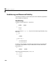
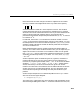
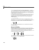
Table Of Contents
- Preface
- Quick Start
- LTI Models
- Introduction
- Creating LTI Models
- LTI Properties
- Model Conversion
- Time Delays
- Simulink Block for LTI Systems
- References
- Operations on LTI Models
- Arrays of LTI Models
- Model Analysis Tools
- The LTI Viewer
- Introduction
- Getting Started Using the LTI Viewer: An Example
- The LTI Viewer Menus
- The Right-Click Menus
- The LTI Viewer Tools Menu
- Simulink LTI Viewer
- Control Design Tools
- The Root Locus Design GUI
- Introduction
- A Servomechanism Example
- Controller Design Using the Root Locus Design GUI
- Additional Root Locus Design GUI Features
- References
- Design Case Studies
- Reliable Computations
- Reference
- Category Tables
- acker
- append
- augstate
- balreal
- bode
- c2d
- canon
- care
- chgunits
- connect
- covar
- ctrb
- ctrbf
- d2c
- d2d
- damp
- dare
- dcgain
- delay2z
- dlqr
- dlyap
- drmodel, drss
- dsort
- dss
- dssdata
- esort
- estim
- evalfr
- feedback
- filt
- frd
- frdata
- freqresp
- gensig
- get
- gram
- hasdelay
- impulse
- initial
- inv
- isct, isdt
- isempty
- isproper
- issiso
- kalman
- kalmd
- lft
- lqgreg
- lqr
- lqrd
- lqry
- lsim
- ltiview
- lyap
- margin
- minreal
- modred
- ndims
- ngrid
- nichols
- norm
- nyquist
- obsv
- obsvf
- ord2
- pade
- parallel
- place
- pole
- pzmap
- reg
- reshape
- rlocfind
- rlocus
- rltool
- rmodel, rss
- series
- set
- sgrid
- sigma
- size
- sminreal
- ss
- ss2ss
- ssbal
- ssdata
- stack
- step
- tf
- tfdata
- totaldelay
- zero
- zgrid
- zpk
- zpkdata
- Index

10 Reliable Computations
10-4
Conditioning and Numerical Stability
Two of the key concepts in numerical anal ysis are the conditioning of problems
and the stability of algorithms.
Conditioning
Consider the linear system given by
A =
0.7800 0.5630
0.9130 0.6590
b =
0.2170
0.2540
Thetruesolutionisx = [1, –1]' and youcan calculateitapproximatelyusing
MATLAB.
x = A\b
x =
1.0000
–1.0000
format long, x
x =
0.99999999991008
–0.99999999987542
Of course, in real problems you almost never have the luxury of knowing the
true solution. This problem is very ill-conditioned. To see this, add a small
perturbation to
A
E =
0.0010 0.0010
–0.0020 –0.0010
and solve the perturbed system
xe = (A+E)\b
xe =
–5.0000
7.3085
Ax b
=
AE
+()
xb
=