
User`s guide
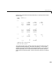
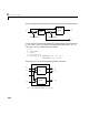
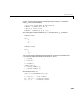
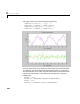
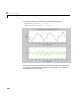
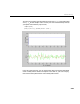
Table Of Contents
- Preface
- Quick Start
- LTI Models
- Introduction
- Creating LTI Models
- LTI Properties
- Model Conversion
- Time Delays
- Simulink Block for LTI Systems
- References
- Operations on LTI Models
- Arrays of LTI Models
- Model Analysis Tools
- The LTI Viewer
- Introduction
- Getting Started Using the LTI Viewer: An Example
- The LTI Viewer Menus
- The Right-Click Menus
- The LTI Viewer Tools Menu
- Simulink LTI Viewer
- Control Design Tools
- The Root Locus Design GUI
- Introduction
- A Servomechanism Example
- Controller Design Using the Root Locus Design GUI
- Additional Root Locus Design GUI Features
- References
- Design Case Studies
- Reliable Computations
- Reference
- Category Tables
- acker
- append
- augstate
- balreal
- bode
- c2d
- canon
- care
- chgunits
- connect
- covar
- ctrb
- ctrbf
- d2c
- d2d
- damp
- dare
- dcgain
- delay2z
- dlqr
- dlyap
- drmodel, drss
- dsort
- dss
- dssdata
- esort
- estim
- evalfr
- feedback
- filt
- frd
- frdata
- freqresp
- gensig
- get
- gram
- hasdelay
- impulse
- initial
- inv
- isct, isdt
- isempty
- isproper
- issiso
- kalman
- kalmd
- lft
- lqgreg
- lqr
- lqrd
- lqry
- lsim
- ltiview
- lyap
- margin
- minreal
- modred
- ndims
- ngrid
- nichols
- norm
- nyquist
- obsv
- obsvf
- ord2
- pade
- parallel
- place
- pole
- pzmap
- reg
- reshape
- rlocfind
- rlocus
- rltool
- rmodel, rss
- series
- set
- sgrid
- sigma
- size
- sminreal
- ss
- ss2ss
- ssbal
- ssdata
- stack
- step
- tf
- tfdata
- totaldelay
- zero
- zgrid
- zpk
- zpkdata
- Index

9 Design Case Studies
9-58
with and as defined on page 9-50, and in the following.
For simplicity, we have dropped the subscripts indicating the time dependence
of the state-space matrices.
Given initial conditions and , you can iterate these equations to
perform the filtering. Note that you must update both the state estimates
and error covariance matrices at each time sample.
Time-Varying Design
Although the Control System Toolbox does not offer specific commands to
perform time-varying Kalman filtering, it is easy to implement the filter
recursions in MATLAB. This section shows how to do this for the stationary
plant considered above.
First generate noisy output measurements
% Use process noise w and measurement noise v generated above
sys = ss(A,B,C,0,–1);
y = lsim(sys,u+w); % w = process noise
yv = + v; % v = measurement noise
Given the initial conditions
x
ˆ
nn 1–[]
x
ˆ
nn[]
Qn[] Ewn[]wn[]
T
()=
Rn[] Evn[]vn[]
T
()=
Pnn[]Exn[] xnn[]–{}xn[] xnn[]–{}
T
()=
Pnn 1–[]Exn[] xnn 1–[]–{}xn[] xnn 1–[]–{}
T
()=
x10
[]
P10
[]
xn.
[]
Pn.
[]
x10[]0,= P10[]BQB
T
=