User`s guide

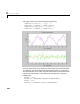
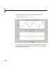
Table Of Contents

9 Design Case Studies

9-56

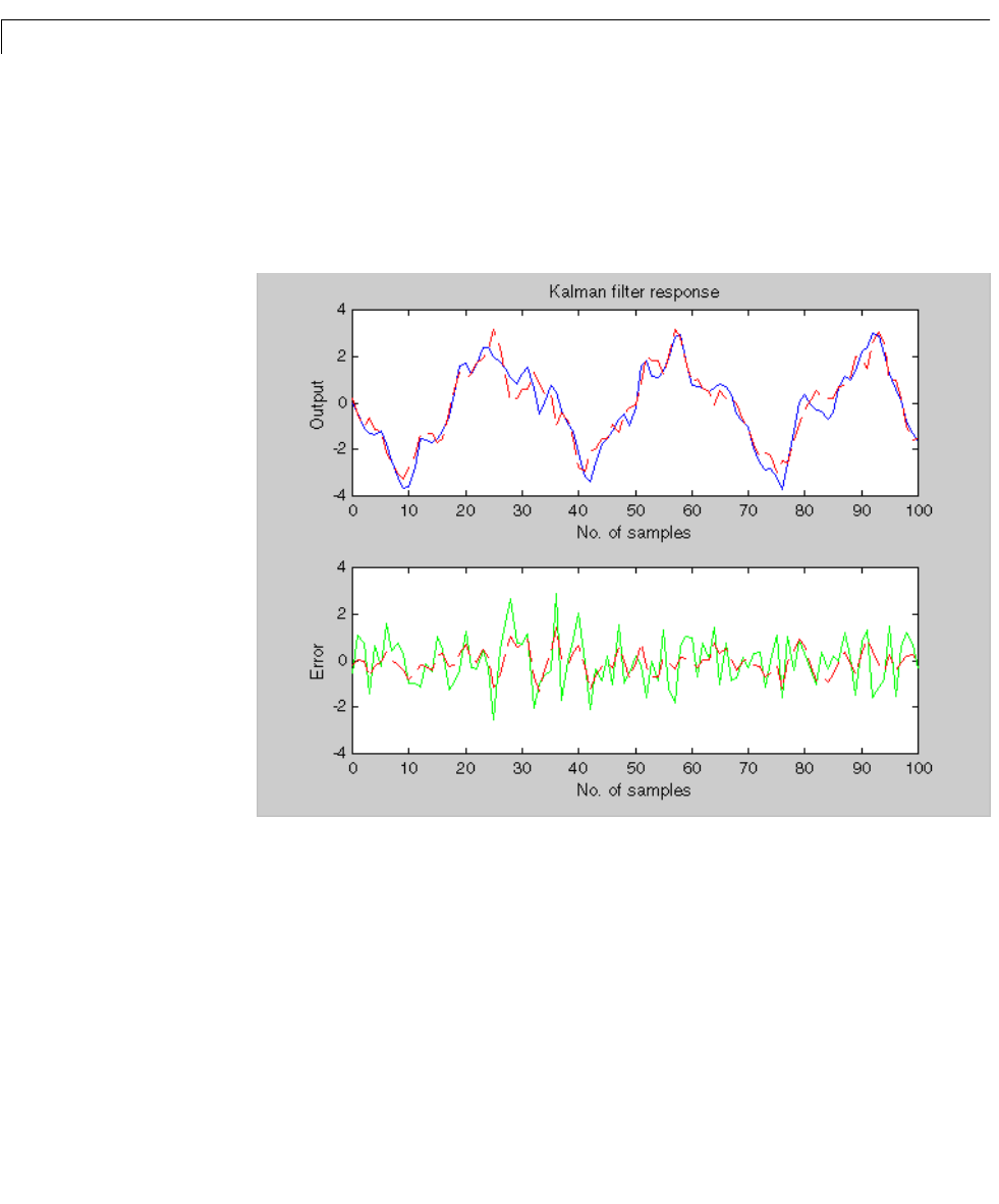
and compare the true and filtered responses graphically.

subplot(211), plot(t,y,'--',t,ye,'-'),

xlabel('No. of samples'), ylabel('Output')

subplot(212), plot(t,y–yv,'-.',t,y–ye,'-'),

xlabel('No. of samples'), ylabel('Error')

The first plot shows the true response (dashed line) a nd the filtered output

(solid line). The second plot compares the measurement error (dash-dot)

with the estimation error (solid). This plot shows that the noise level has been

significantly reduced. This is confirmed by the following error covariance

computations.

MeasErr = y–yv;

MeasErrCov = sum(MeasErr.*MeasErr)/length(MeasErr);

EstErr = y–ye;

EstErrCov = sum(EstErr.*EstErr)/length(EstErr);