
User`s guide
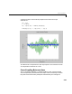
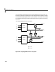
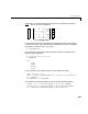
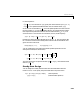
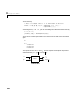
Table Of Contents
- Preface
- Quick Start
- LTI Models
- Introduction
- Creating LTI Models
- LTI Properties
- Model Conversion
- Time Delays
- Simulink Block for LTI Systems
- References
- Operations on LTI Models
- Arrays of LTI Models
- Model Analysis Tools
- The LTI Viewer
- Introduction
- Getting Started Using the LTI Viewer: An Example
- The LTI Viewer Menus
- The Right-Click Menus
- The LTI Viewer Tools Menu
- Simulink LTI Viewer
- Control Design Tools
- The Root Locus Design GUI
- Introduction
- A Servomechanism Example
- Controller Design Using the Root Locus Design GUI
- Additional Root Locus Design GUI Features
- References
- Design Case Studies
- Reliable Computations
- Reference
- Category Tables
- acker
- append
- augstate
- balreal
- bode
- c2d
- canon
- care
- chgunits
- connect
- covar
- ctrb
- ctrbf
- d2c
- d2d
- damp
- dare
- dcgain
- delay2z
- dlqr
- dlyap
- drmodel, drss
- dsort
- dss
- dssdata
- esort
- estim
- evalfr
- feedback
- filt
- frd
- frdata
- freqresp
- gensig
- get
- gram
- hasdelay
- impulse
- initial
- inv
- isct, isdt
- isempty
- isproper
- issiso
- kalman
- kalmd
- lft
- lqgreg
- lqr
- lqrd
- lqry
- lsim
- ltiview
- lyap
- margin
- minreal
- modred
- ndims
- ngrid
- nichols
- norm
- nyquist
- obsv
- obsvf
- ord2
- pade
- parallel
- place
- pole
- pzmap
- reg
- reshape
- rlocfind
- rlocus
- rltool
- rmodel, rss
- series
- set
- sgrid
- sigma
- size
- sminreal
- ss
- ss2ss
- ssbal
- ssdata
- stack
- step
- tf
- tfdata
- totaldelay
- zero
- zgrid
- zpk
- zpkdata
- Index

9 Design Case Studies
9-50
Kalman Filtering
This final case study illustrates the use of the Control System Toolbox for
Kalman filter design and simulation. Both steady-state and time-varying
Kalman filters are considered.
Consider the discrete plant
with additive Gaussian noise on the input and data
A = [1.1269 –0.4940 0.1129
1.0000 0 0
0 1.0000 0];
B = [–0.3832
0.5919
0.5191];
C = [1 0 0];
Our goal is to design a Kalman filter that estimates the output given the
inputs and the noisy o utput measurements
where is some Gaussian white noise.
Discrete Kalman Filter
The equations of the steady-state Kalman filter for this problem are given as
follows.
Measurement update
Time update
xn 1
+[]
Ax n
[]
Bun
[]
wn
[]+()+=
yn[] Cx n[]=
wn
[]
un
[]
yn
[]
un
[]
y
v
n
[]
Cx n
[]
vn
[]+=
vn
[]
x
ˆ
nn[]x
ˆ
nn 1–[]My
v
n[] Cx
ˆ
nn 1–[]–()+=
x
ˆ
n1n+[]Ax
ˆ
nn[]Bu n[]+=