
User`s guide
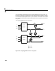
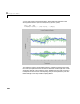
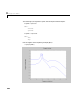
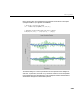
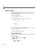
Table Of Contents
- Preface
- Quick Start
- LTI Models
- Introduction
- Creating LTI Models
- LTI Properties
- Model Conversion
- Time Delays
- Simulink Block for LTI Systems
- References
- Operations on LTI Models
- Arrays of LTI Models
- Model Analysis Tools
- The LTI Viewer
- Introduction
- Getting Started Using the LTI Viewer: An Example
- The LTI Viewer Menus
- The Right-Click Menus
- The LTI Viewer Tools Menu
- Simulink LTI Viewer
- Control Design Tools
- The Root Locus Design GUI
- Introduction
- A Servomechanism Example
- Controller Design Using the Root Locus Design GUI
- Additional Root Locus Design GUI Features
- References
- Design Case Studies
- Reliable Computations
- Reference
- Category Tables
- acker
- append
- augstate
- balreal
- bode
- c2d
- canon
- care
- chgunits
- connect
- covar
- ctrb
- ctrbf
- d2c
- d2d
- damp
- dare
- dcgain
- delay2z
- dlqr
- dlyap
- drmodel, drss
- dsort
- dss
- dssdata
- esort
- estim
- evalfr
- feedback
- filt
- frd
- frdata
- freqresp
- gensig
- get
- gram
- hasdelay
- impulse
- initial
- inv
- isct, isdt
- isempty
- isproper
- issiso
- kalman
- kalmd
- lft
- lqgreg
- lqr
- lqrd
- lqry
- lsim
- ltiview
- lyap
- margin
- minreal
- modred
- ndims
- ngrid
- nichols
- norm
- nyquist
- obsv
- obsvf
- ord2
- pade
- parallel
- place
- pole
- pzmap
- reg
- reshape
- rlocfind
- rlocus
- rltool
- rmodel, rss
- series
- set
- sgrid
- sigma
- size
- sminreal
- ss
- ss2ss
- ssbal
- ssdata
- stack
- step
- tf
- tfdata
- totaldelay
- zero
- zgrid
- zpk
- zpkdata
- Index
LQG Regulation
9-45
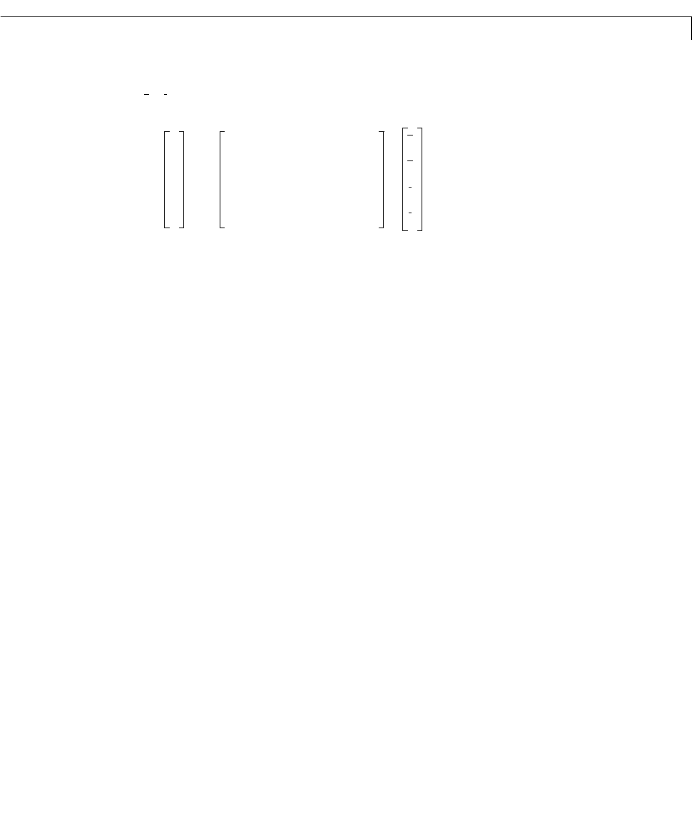
Accordingly, the thickness gaps and rolling forces are related to the outputs
of the - and -axis models by
Let’s see how the previous “decoupled” LQG design fares when cross-coupling
is takeninto account.Tobuild the two-axesmodel shown inFigure 9-2, append
the models
Px and Py for the - and -axes.
P = append(Px,Py)
For convenience, reorder the inputs and outputs so that the commands and
thickness gaps appear first.
P = P([1 3 2 4],[1 4 2 3 5 6])
P.outputname
ans =
'x-gap'
'y-gap'
'x-force'
'y-force'
Finally, place the cross-coupling matrix in series with the outputs.
gxy = 0.1; gyx = 0.4;
CCmat = [eye(2) [0 gyx*gx;gxy*gy 0] ; zeros(2) [1 –gyx;–gxy 1]]
Pc = CCmat * P
Pc.outputname = P.outputname
To simulate the closed-loop response, also form the closed-loop model by
feedin = 1:2 % first two inputs of Pc are the commands
feedout = 3:4 % last two outputs of Pc are the measurements
cl = feedback(Pc,append(Regx,Regy),feedin,feedout,+1)
δ
x
f
x
...,,
x
y
δ
x
δ
y
f
x
f
y
100g
yx
g
x
01g
xy
g
y
0
001g
yx
–
00g
xy
– 1
δ
x
δ
y
f
x
f
y
=
cross-coupling matrix
x
y