
User`s guide
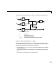
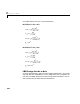
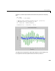
Table Of Contents
- Preface
- Quick Start
- LTI Models
- Introduction
- Creating LTI Models
- LTI Properties
- Model Conversion
- Time Delays
- Simulink Block for LTI Systems
- References
- Operations on LTI Models
- Arrays of LTI Models
- Model Analysis Tools
- The LTI Viewer
- Introduction
- Getting Started Using the LTI Viewer: An Example
- The LTI Viewer Menus
- The Right-Click Menus
- The LTI Viewer Tools Menu
- Simulink LTI Viewer
- Control Design Tools
- The Root Locus Design GUI
- Introduction
- A Servomechanism Example
- Controller Design Using the Root Locus Design GUI
- Additional Root Locus Design GUI Features
- References
- Design Case Studies
- Reliable Computations
- Reference
- Category Tables
- acker
- append
- augstate
- balreal
- bode
- c2d
- canon
- care
- chgunits
- connect
- covar
- ctrb
- ctrbf
- d2c
- d2d
- damp
- dare
- dcgain
- delay2z
- dlqr
- dlyap
- drmodel, drss
- dsort
- dss
- dssdata
- esort
- estim
- evalfr
- feedback
- filt
- frd
- frdata
- freqresp
- gensig
- get
- gram
- hasdelay
- impulse
- initial
- inv
- isct, isdt
- isempty
- isproper
- issiso
- kalman
- kalmd
- lft
- lqgreg
- lqr
- lqrd
- lqry
- lsim
- ltiview
- lyap
- margin
- minreal
- modred
- ndims
- ngrid
- nichols
- norm
- nyquist
- obsv
- obsvf
- ord2
- pade
- parallel
- place
- pole
- pzmap
- reg
- reshape
- rlocfind
- rlocus
- rltool
- rmodel, rss
- series
- set
- sgrid
- sigma
- size
- sminreal
- ss
- ss2ss
- ssbal
- ssdata
- stack
- step
- tf
- tfdata
- totaldelay
- zero
- zgrid
- zpk
- zpkdata
- Index

LQG Regulation
9-35
Start with the -axis. First specify the model components as transfer function
objects .
% Hydraulic actuator (with input "u-x")
Hx = tf(2.4e8,[1 72 90^2],'inputname','u-x')
% Input thickness/hardness disturbance model
Fix = tf(1e4,[1 0.05],'inputn','w-ix')
% Rolling eccentricity model
Fex = tf([3e4 0],[1 0.125 6^2],'inputn','w-ex')
% Gain from force to thickness gap
gx = 1e–6;
Next build the open-loop model shown in Figure 9-1 above. You could use the
function
connect for this purpose, but it is easier to build this model by
elementary
append and series connections.
% I/O map from inputs to forces f1 and f2
Px = append([ss(Hx) Fex],Fix)
% Add static gain from f1,f2 to outputs ”x-gap” and ”x-force”
Px = [–gx gx;1 1] * Px
% Give names to the outputs:
set(Px,'outputn',{'x-gap' 'x-force'})
Note: To obtain minimal state-space realizations, always convert transfer
function models to state space before connecting them. Combining transfer
functions and then converting to state space may produce nonminimal
state-space models.
x