
User`s guide
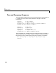
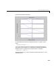

Table Of Contents
- Preface
- Quick Start
- LTI Models
- Introduction
- Creating LTI Models
- LTI Properties
- Model Conversion
- Time Delays
- Simulink Block for LTI Systems
- References
- Operations on LTI Models
- Arrays of LTI Models
- Model Analysis Tools
- The LTI Viewer
- Introduction
- Getting Started Using the LTI Viewer: An Example
- The LTI Viewer Menus
- The Right-Click Menus
- The LTI Viewer Tools Menu
- Simulink LTI Viewer
- Control Design Tools
- The Root Locus Design GUI
- Introduction
- A Servomechanism Example
- Controller Design Using the Root Locus Design GUI
- Additional Root Locus Design GUI Features
- References
- Design Case Studies
- Reliable Computations
- Reference
- Category Tables
- acker
- append
- augstate
- balreal
- bode
- c2d
- canon
- care
- chgunits
- connect
- covar
- ctrb
- ctrbf
- d2c
- d2d
- damp
- dare
- dcgain
- delay2z
- dlqr
- dlyap
- drmodel, drss
- dsort
- dss
- dssdata
- esort
- estim
- evalfr
- feedback
- filt
- frd
- frdata
- freqresp
- gensig
- get
- gram
- hasdelay
- impulse
- initial
- inv
- isct, isdt
- isempty
- isproper
- issiso
- kalman
- kalmd
- lft
- lqgreg
- lqr
- lqrd
- lqry
- lsim
- ltiview
- lyap
- margin
- minreal
- modred
- ndims
- ngrid
- nichols
- norm
- nyquist
- obsv
- obsvf
- ord2
- pade
- parallel
- place
- pole
- pzmap
- reg
- reshape
- rlocfind
- rlocus
- rltool
- rmodel, rss
- series
- set
- sgrid
- sigma
- size
- sminreal
- ss
- ss2ss
- ssbal
- ssdata
- stack
- step
- tf
- tfdata
- totaldelay
- zero
- zgrid
- zpk
- zpkdata
- Index

1 Quick Start
1-14
Time and Frequency Response
Thefollowingcommandsproducevarioustimeandfrequencyresponseplotsfor
LTI models (see “Time and Frequency Response” on page 5-9 for more
information).
step(sys) % step response
impulse(sys) % impulse response
initial(sys,x0) % undriven response to initial condition
lsim(sys,u,t,x0) % response to input u
bode(sys) % Bode plot
nyquist(sys) % Nyquist plot
nichols(sys) % Nichols plot
sigma(sys) % singular value plot
freqresp(sys,w) % complex frequency response
These commands work for both continuous- and discrete-time LTI models sys
without restriction on the number of inputs or outputs. For MIMO systems,
they produce an array of plots with one plot per I/O channel. For example,
sys = [tf(1,[1 1]) 1 ; tf([1 5],[1 1 10]) tf(–1,[1 0])];
bode(sys)