
User`s guide
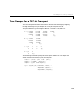

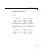
Table Of Contents
- Preface
- Quick Start
- LTI Models
- Introduction
- Creating LTI Models
- LTI Properties
- Model Conversion
- Time Delays
- Simulink Block for LTI Systems
- References
- Operations on LTI Models
- Arrays of LTI Models
- Model Analysis Tools
- The LTI Viewer
- Introduction
- Getting Started Using the LTI Viewer: An Example
- The LTI Viewer Menus
- The Right-Click Menus
- The LTI Viewer Tools Menu
- Simulink LTI Viewer
- Control Design Tools
- The Root Locus Design GUI
- Introduction
- A Servomechanism Example
- Controller Design Using the Root Locus Design GUI
- Additional Root Locus Design GUI Features
- References
- Design Case Studies
- Reliable Computations
- Reference
- Category Tables
- acker
- append
- augstate
- balreal
- bode
- c2d
- canon
- care
- chgunits
- connect
- covar
- ctrb
- ctrbf
- d2c
- d2d
- damp
- dare
- dcgain
- delay2z
- dlqr
- dlyap
- drmodel, drss
- dsort
- dss
- dssdata
- esort
- estim
- evalfr
- feedback
- filt
- frd
- frdata
- freqresp
- gensig
- get
- gram
- hasdelay
- impulse
- initial
- inv
- isct, isdt
- isempty
- isproper
- issiso
- kalman
- kalmd
- lft
- lqgreg
- lqr
- lqrd
- lqry
- lsim
- ltiview
- lyap
- margin
- minreal
- modred
- ndims
- ngrid
- nichols
- norm
- nyquist
- obsv
- obsvf
- ord2
- pade
- parallel
- place
- pole
- pzmap
- reg
- reshape
- rlocfind
- rlocus
- rltool
- rmodel, rss
- series
- set
- sgrid
- sigma
- size
- sminreal
- ss
- ss2ss
- ssbal
- ssdata
- stack
- step
- tf
- tfdata
- totaldelay
- zero
- zgrid
- zpk
- zpkdata
- Index

Yaw Damper for a 747 Jet Transport
9-3
Yaw Damper for a 747 Jet Transport
This case study demonstrates the tools for classical control design by stepping
through the design of a yaw damper for a 747 jet transport aircraft.
The jet model during cruise flight at MACH = 0.8 and H = 40,000 ft. is
A = [–0.0558 –0.9968 0.0802 0.0415
0.5980 –0.1150 –0.0318 0
–3.0500 0.3880 –0.4650 0
0 0.0805 1.0000 0];
B = [ 0.0729 0.0000
–4.7500 0.00775
1.5300 0.1430
0 0];
C = [0 1 0 0
0 0 0 1];
D = [0 0
0 0];
The following commands specify this state-space model as an LTI object and
attach names to t he states, inputs, and outputs.
states = {'beta' 'yaw' 'roll' 'phi'};
inputs = {'rudder' 'aileron'};
output = {'yaw' 'bank angle'};
sys = ss(A,B,C,D,'statename',states,...
'inputname',inputs,...
'outputname',outputs);