
User`s guide
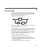
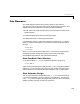
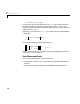
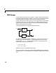
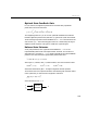
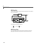

Table Of Contents
- Preface
- Quick Start
- LTI Models
- Introduction
- Creating LTI Models
- LTI Properties
- Model Conversion
- Time Delays
- Simulink Block for LTI Systems
- References
- Operations on LTI Models
- Arrays of LTI Models
- Model Analysis Tools
- The LTI Viewer
- Introduction
- Getting Started Using the LTI Viewer: An Example
- The LTI Viewer Menus
- The Right-Click Menus
- The LTI Viewer Tools Menu
- Simulink LTI Viewer
- Control Design Tools
- The Root Locus Design GUI
- Introduction
- A Servomechanism Example
- Controller Design Using the Root Locus Design GUI
- Additional Root Locus Design GUI Features
- References
- Design Case Studies
- Reliable Computations
- Reference
- Category Tables
- acker
- append
- augstate
- balreal
- bode
- c2d
- canon
- care
- chgunits
- connect
- covar
- ctrb
- ctrbf
- d2c
- d2d
- damp
- dare
- dcgain
- delay2z
- dlqr
- dlyap
- drmodel, drss
- dsort
- dss
- dssdata
- esort
- estim
- evalfr
- feedback
- filt
- frd
- frdata
- freqresp
- gensig
- get
- gram
- hasdelay
- impulse
- initial
- inv
- isct, isdt
- isempty
- isproper
- issiso
- kalman
- kalmd
- lft
- lqgreg
- lqr
- lqrd
- lqry
- lsim
- ltiview
- lyap
- margin
- minreal
- modred
- ndims
- ngrid
- nichols
- norm
- nyquist
- obsv
- obsvf
- ord2
- pade
- parallel
- place
- pole
- pzmap
- reg
- reshape
- rlocfind
- rlocus
- rltool
- rmodel, rss
- series
- set
- sgrid
- sigma
- size
- sminreal
- ss
- ss2ss
- ssbal
- ssdata
- stack
- step
- tf
- tfdata
- totaldelay
- zero
- zgrid
- zpk
- zpkdata
- Index

Pole Placement
7-5
Pole Placement
The closed-loop pole locations have a direct impact on time response
characteristics such as rise time, settling time, and transient oscillations. This
suggests the following method for tuning the closed-loop behavior:
1 Based on the time response specifications, select desirable locations for the
closed -loop poles.
2 Compute feedback gains that achieve these locations.
This design technique is known as pole placement.
Pole placement requires a state-space model of the system (use
ss to convert
other LTI models to state space). In continuous time, this model should be of
the form
where i s the vector of control inputs and is the vector of measurements.
Designing a dynamic compensator for this system involves two steps:
state-feedback gain selection, and state estimator design.
State-Feedback Gain Selection
Under state feedback , the closed-loop dynamics are given by
and the closed-loop poles are the eigenvalues of . Using pole placement
algorithms, you can compute a gain matrix that assigns these poles to any
desired locations in the complex p lane (provided that is controllable).
State Estimator Design
You cannot implement the state-feed back law unless the full st at e
is mea su r e d. Howev er, you can cons tru ct a state estimate such that the
law retains the same pole assignmentproperties. This is a chieved by
designing a state estimator (or observer) of the form
x
·
Ax Bu+=
yCxDu+=
u
y
uKx
–=
x
·
ABK–()x=
ABK
–
K
AB
,()
uKx
–=
x
ξ
uK
ξ–=