
User`s guide
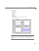
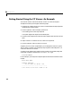
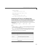
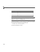
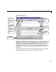
Table Of Contents
- Preface
- Quick Start
- LTI Models
- Introduction
- Creating LTI Models
- LTI Properties
- Model Conversion
- Time Delays
- Simulink Block for LTI Systems
- References
- Operations on LTI Models
- Arrays of LTI Models
- Model Analysis Tools
- The LTI Viewer
- Introduction
- Getting Started Using the LTI Viewer: An Example
- The LTI Viewer Menus
- The Right-Click Menus
- The LTI Viewer Tools Menu
- Simulink LTI Viewer
- Control Design Tools
- The Root Locus Design GUI
- Introduction
- A Servomechanism Example
- Controller Design Using the Root Locus Design GUI
- Additional Root Locus Design GUI Features
- References
- Design Case Studies
- Reliable Computations
- Reference
- Category Tables
- acker
- append
- augstate
- balreal
- bode
- c2d
- canon
- care
- chgunits
- connect
- covar
- ctrb
- ctrbf
- d2c
- d2d
- damp
- dare
- dcgain
- delay2z
- dlqr
- dlyap
- drmodel, drss
- dsort
- dss
- dssdata
- esort
- estim
- evalfr
- feedback
- filt
- frd
- frdata
- freqresp
- gensig
- get
- gram
- hasdelay
- impulse
- initial
- inv
- isct, isdt
- isempty
- isproper
- issiso
- kalman
- kalmd
- lft
- lqgreg
- lqr
- lqrd
- lqry
- lsim
- ltiview
- lyap
- margin
- minreal
- modred
- ndims
- ngrid
- nichols
- norm
- nyquist
- obsv
- obsvf
- ord2
- pade
- parallel
- place
- pole
- pzmap
- reg
- reshape
- rlocfind
- rlocus
- rltool
- rmodel, rss
- series
- set
- sgrid
- sigma
- size
- sminreal
- ss
- ss2ss
- ssbal
- ssdata
- stack
- step
- tf
- tfdata
- totaldelay
- zero
- zgrid
- zpk
- zpkdata
- Index

Getting Started Using the LTI Viewer: An Example
6-5
Transfer function:
2 s^3 + 1.2 s^2 + 15.1 s + 7.5
----------------------------------------
s^4 + 2.12 s^3 + 10.2 s^2 + 15.1 s + 7.5
Transfer function:
1.2 s^3 + 1.12 s^2 + 9.1 s + 7.5
----------------------------------------
s^4 + 1.32 s^3 + 10.12 s^2 + 9.1 s + 7.5
Initializing the LTI Viewer with Multiple Plots
For a given LTI model, you ca n use the LTI Viewer to simultaneously display
multiple response plot types, such as the Bode plot and the step response. You
can also initialize the LTI Viewer to display the plots of several different
models at once. The general syntax for initializing the LTI Viewer to plot up to
six plot types is
ltiview({'type1';'type2';...;'typek'},sys1,...,sysn)
where:
•
{'type1';'type2';...;'typek'} is a cell array listing up to six strings for
the names of the plot types ( ).
•
sys1, ..., sysn is a list of the MATLAB workspace variable names for the
systems whose responses you want to initially display in the LTI Viewer.
Theplottypenamescanbeanyofthefollowing.
Plot Type Description
bode
Bode plot
impulse
Impulse response
initial
Initial state response for SS models
lsim
LTI model response to general input
nichols
Nichols chart
nyquist
Nyquist plo t
k
6
≤