
User`s guide
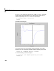
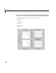
Table Of Contents
- Preface
- Quick Start
- LTI Models
- Introduction
- Creating LTI Models
- LTI Properties
- Model Conversion
- Time Delays
- Simulink Block for LTI Systems
- References
- Operations on LTI Models
- Arrays of LTI Models
- Model Analysis Tools
- The LTI Viewer
- Introduction
- Getting Started Using the LTI Viewer: An Example
- The LTI Viewer Menus
- The Right-Click Menus
- The LTI Viewer Tools Menu
- Simulink LTI Viewer
- Control Design Tools
- The Root Locus Design GUI
- Introduction
- A Servomechanism Example
- Controller Design Using the Root Locus Design GUI
- Additional Root Locus Design GUI Features
- References
- Design Case Studies
- Reliable Computations
- Reference
- Category Tables
- acker
- append
- augstate
- balreal
- bode
- c2d
- canon
- care
- chgunits
- connect
- covar
- ctrb
- ctrbf
- d2c
- d2d
- damp
- dare
- dcgain
- delay2z
- dlqr
- dlyap
- drmodel, drss
- dsort
- dss
- dssdata
- esort
- estim
- evalfr
- feedback
- filt
- frd
- frdata
- freqresp
- gensig
- get
- gram
- hasdelay
- impulse
- initial
- inv
- isct, isdt
- isempty
- isproper
- issiso
- kalman
- kalmd
- lft
- lqgreg
- lqr
- lqrd
- lqry
- lsim
- ltiview
- lyap
- margin
- minreal
- modred
- ndims
- ngrid
- nichols
- norm
- nyquist
- obsv
- obsvf
- ord2
- pade
- parallel
- place
- pole
- pzmap
- reg
- reshape
- rlocfind
- rlocus
- rltool
- rmodel, rss
- series
- set
- sgrid
- sigma
- size
- sminreal
- ss
- ss2ss
- ssbal
- ssdata
- stack
- step
- tf
- tfdata
- totaldelay
- zero
- zgrid
- zpk
- zpkdata
- Index

5 Model Analysis Tools
5-14
several LTI models on a single plot. To do so, invoke the corresponding
command line function using the list
sys1,..., sysN of models as the inputs.
step(sys1,sys2,...,sysN)
impulse(sys1,sys2,...,sysN)
...
bode(sys1,sys2,...,sysN)
nichols(sys1,sys2,...,sysN)
...
All models in the argument lists of any of the response plotting functions
(except for
sigma) must have the same number of inputs and outputs. To
differentiate the plots easily, you can also specify a distinctive color/linestyle/
marker for each system just as you would wit h the
plot command. For
example,
bode(sys1,’r’,sys2,’y--’,sys3,’gx’)
plots sys1 with solid red lines, sys2 with yellow dashed lines, and sys3 with
green
x markers.
You can plot responses of multiple modelso n the same plot. These models need
not be all continuous-time or all discrete-time.