
User`s guide
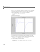
Table Of Contents
- Preface
- Quick Start
- LTI Models
- Introduction
- Creating LTI Models
- LTI Properties
- Model Conversion
- Time Delays
- Simulink Block for LTI Systems
- References
- Operations on LTI Models
- Arrays of LTI Models
- Model Analysis Tools
- The LTI Viewer
- Introduction
- Getting Started Using the LTI Viewer: An Example
- The LTI Viewer Menus
- The Right-Click Menus
- The LTI Viewer Tools Menu
- Simulink LTI Viewer
- Control Design Tools
- The Root Locus Design GUI
- Introduction
- A Servomechanism Example
- Controller Design Using the Root Locus Design GUI
- Additional Root Locus Design GUI Features
- References
- Design Case Studies
- Reliable Computations
- Reference
- Category Tables
- acker
- append
- augstate
- balreal
- bode
- c2d
- canon
- care
- chgunits
- connect
- covar
- ctrb
- ctrbf
- d2c
- d2d
- damp
- dare
- dcgain
- delay2z
- dlqr
- dlyap
- drmodel, drss
- dsort
- dss
- dssdata
- esort
- estim
- evalfr
- feedback
- filt
- frd
- frdata
- freqresp
- gensig
- get
- gram
- hasdelay
- impulse
- initial
- inv
- isct, isdt
- isempty
- isproper
- issiso
- kalman
- kalmd
- lft
- lqgreg
- lqr
- lqrd
- lqry
- lsim
- ltiview
- lyap
- margin
- minreal
- modred
- ndims
- ngrid
- nichols
- norm
- nyquist
- obsv
- obsvf
- ord2
- pade
- parallel
- place
- pole
- pzmap
- reg
- reshape
- rlocfind
- rlocus
- rltool
- rmodel, rss
- series
- set
- sgrid
- sigma
- size
- sminreal
- ss
- ss2ss
- ssbal
- ssdata
- stack
- step
- tf
- tfdata
- totaldelay
- zero
- zgrid
- zpk
- zpkdata
- Index

Time and Frequency Response
5-11
Note: When specifying a time vector t = [0:dt:tf],rememberthe
following constraints on the spacing
dt between time samples:
• For discrete systems,
dt should match the system sample time.
• Continuous systems are first discretized using zero-order hold and
dt as
sampling period, and
step simulates t he resulting discrete system. As a
result, you should pick
dt small enough to capture the main features of the
continuous transient response.
The syntax step(sys) automatically takes these issues into account.
Finally, the function
lsim simulatestheresponsetomoregeneralclassesof
inputs. For example,
t = 0:0.01:10
u = sin(t)
lsim(sys,u,t)
simulates the zero-initial condition response of the LTI system sys to a sine
wave for a duration of 10 seconds.
Note: You can also implement several plotting options by using the
right-click menus accessible from the (white) plot region of all time and
frequency plots. These options are listed on the menu. To learn more about the
right-click menus on plots, see “The Right-Click Menus” on page 6-18
Frequency Response
The Control System Toolbox provides response-plotting functions for the
following frequency domain analysis tools:
• Bode plots
• Nichols charts
• Nyquist plots
• Singular value plots