
User`s guide
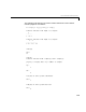
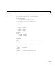
Table Of Contents
- Preface
- Quick Start
- LTI Models
- Introduction
- Creating LTI Models
- LTI Properties
- Model Conversion
- Time Delays
- Simulink Block for LTI Systems
- References
- Operations on LTI Models
- Arrays of LTI Models
- Model Analysis Tools
- The LTI Viewer
- Introduction
- Getting Started Using the LTI Viewer: An Example
- The LTI Viewer Menus
- The Right-Click Menus
- The LTI Viewer Tools Menu
- Simulink LTI Viewer
- Control Design Tools
- The Root Locus Design GUI
- Introduction
- A Servomechanism Example
- Controller Design Using the Root Locus Design GUI
- Additional Root Locus Design GUI Features
- References
- Design Case Studies
- Reliable Computations
- Reference
- Category Tables
- acker
- append
- augstate
- balreal
- bode
- c2d
- canon
- care
- chgunits
- connect
- covar
- ctrb
- ctrbf
- d2c
- d2d
- damp
- dare
- dcgain
- delay2z
- dlqr
- dlyap
- drmodel, drss
- dsort
- dss
- dssdata
- esort
- estim
- evalfr
- feedback
- filt
- frd
- frdata
- freqresp
- gensig
- get
- gram
- hasdelay
- impulse
- initial
- inv
- isct, isdt
- isempty
- isproper
- issiso
- kalman
- kalmd
- lft
- lqgreg
- lqr
- lqrd
- lqry
- lsim
- ltiview
- lyap
- margin
- minreal
- modred
- ndims
- ngrid
- nichols
- norm
- nyquist
- obsv
- obsvf
- ord2
- pade
- parallel
- place
- pole
- pzmap
- reg
- reshape
- rlocfind
- rlocus
- rltool
- rmodel, rss
- series
- set
- sgrid
- sigma
- size
- sminreal
- ss
- ss2ss
- ssbal
- ssdata
- stack
- step
- tf
- tfdata
- totaldelay
- zero
- zgrid
- zpk
- zpkdata
- Index

5 Model Analysis Tools
5-6
Thesefunctionsalsoo perateonLTIarraysandreturnarrays.F or example,the
poles of a three dimensional LTI array
sysarray are obtained as follows.
sysarray = tf(rss(2,1,1,3))
Model sysarray(:,:,1,1)
=======================
Transfer function:
-0.6201 s - 1.905
---------------------
s^2 + 5.672 s + 7.405
Model sysarray(:,:,2,1)
=======================
Transfer function:
0.4282 s^2 + 0.3706 s + 0.04264
-------------------------------
s^2 + 1.056 s + 0.1719
Model sysarray(:,:,3,1)
=======================
Transfer function:
0.621 s + 0.7567
---------------------
s^2 + 2.942 s + 2.113
3x1 array of continuous-time transfer functions.
pole(sysarray)
ans(:,:,1) =
-3.6337
-2.0379
ans(:,:,2) =
-0.8549
-0.2011
ans(:,:,3) =
-1.6968
-1.2452