
User`s guide
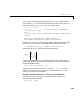
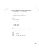

Table Of Contents
- Preface
- Quick Start
- LTI Models
- Introduction
- Creating LTI Models
- LTI Properties
- Model Conversion
- Time Delays
- Simulink Block for LTI Systems
- References
- Operations on LTI Models
- Arrays of LTI Models
- Model Analysis Tools
- The LTI Viewer
- Introduction
- Getting Started Using the LTI Viewer: An Example
- The LTI Viewer Menus
- The Right-Click Menus
- The LTI Viewer Tools Menu
- Simulink LTI Viewer
- Control Design Tools
- The Root Locus Design GUI
- Introduction
- A Servomechanism Example
- Controller Design Using the Root Locus Design GUI
- Additional Root Locus Design GUI Features
- References
- Design Case Studies
- Reliable Computations
- Reference
- Category Tables
- acker
- append
- augstate
- balreal
- bode
- c2d
- canon
- care
- chgunits
- connect
- covar
- ctrb
- ctrbf
- d2c
- d2d
- damp
- dare
- dcgain
- delay2z
- dlqr
- dlyap
- drmodel, drss
- dsort
- dss
- dssdata
- esort
- estim
- evalfr
- feedback
- filt
- frd
- frdata
- freqresp
- gensig
- get
- gram
- hasdelay
- impulse
- initial
- inv
- isct, isdt
- isempty
- isproper
- issiso
- kalman
- kalmd
- lft
- lqgreg
- lqr
- lqrd
- lqry
- lsim
- ltiview
- lyap
- margin
- minreal
- modred
- ndims
- ngrid
- nichols
- norm
- nyquist
- obsv
- obsvf
- ord2
- pade
- parallel
- place
- pole
- pzmap
- reg
- reshape
- rlocfind
- rlocus
- rltool
- rmodel, rss
- series
- set
- sgrid
- sigma
- size
- sminreal
- ss
- ss2ss
- ssbal
- ssdata
- stack
- step
- tf
- tfdata
- totaldelay
- zero
- zgrid
- zpk
- zpkdata
- Index

Operations on LTI Arrays
4-29
You can do this efficiently by first setting up an LTI array h containing the
SISO models and then using concatenation to form the LTI array
H of
MIMO LTI models , . To do this, type
tau = [1.1 1.2 1.3];
for i=1:3 % Form LTI array h of SISO models.
h(:,:,i)=tf(1,[1 tau]);
end
H = [h 0; –1 tf(1,[1 0])]; %Concatenation: array h & single models
size(H)
3x1 array of continuous-time transfer functions
Each transfer function has 2 output(s) and 2 input(s).
Similarly, you can use append to perform the diagonal appending of each model
in the SISO LTI array
h with a fixed single (SISO or MIMO) LTI model.
S = append(h,tf(1,[1 3])); % Append a single model to h.
specifies an LTI array S in which each model has the form
You can also combine an LTI array of MIMO models and a single MIMO LTI
model using arithmetic operations. For example, if
h is the LTI array of three
SISO models defined above,
[h,h] + [tf(1,[1 0]);tf(1,[1 5])]
adds the single one-output, two-input LTI model [1/s 1/(s + 5)] to every
model in the 3-by-1 LTI array of one-output, two-input models
[h,h].The
result is a new 3-by-2 array of models.
Examples: Arithmetic Operations on LTI Arrays and SISO Models
Using the LTI array of one-output, two-input state-space models [h,h],
defined in the previous example,
tf(1,[1 3]) + [h,h]
1 s
τ+(
)
⁄
H
τ
s
(
)
τ
1.1 1.2 1.3
,,{}∈
S
τ
s()
1
s τ+
-----------
0
0
1
s 3+
------------
=