
User`s guide
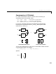
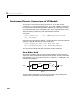
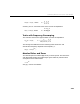
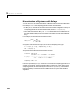

Table Of Contents
- Preface
- Quick Start
- LTI Models
- Introduction
- Creating LTI Models
- LTI Properties
- Model Conversion
- Time Delays
- Simulink Block for LTI Systems
- References
- Operations on LTI Models
- Arrays of LTI Models
- Model Analysis Tools
- The LTI Viewer
- Introduction
- Getting Started Using the LTI Viewer: An Example
- The LTI Viewer Menus
- The Right-Click Menus
- The LTI Viewer Tools Menu
- Simulink LTI Viewer
- Control Design Tools
- The Root Locus Design GUI
- Introduction
- A Servomechanism Example
- Controller Design Using the Root Locus Design GUI
- Additional Root Locus Design GUI Features
- References
- Design Case Studies
- Reliable Computations
- Reference
- Category Tables
- acker
- append
- augstate
- balreal
- bode
- c2d
- canon
- care
- chgunits
- connect
- covar
- ctrb
- ctrbf
- d2c
- d2d
- damp
- dare
- dcgain
- delay2z
- dlqr
- dlyap
- drmodel, drss
- dsort
- dss
- dssdata
- esort
- estim
- evalfr
- feedback
- filt
- frd
- frdata
- freqresp
- gensig
- get
- gram
- hasdelay
- impulse
- initial
- inv
- isct, isdt
- isempty
- isproper
- issiso
- kalman
- kalmd
- lft
- lqgreg
- lqr
- lqrd
- lqry
- lsim
- ltiview
- lyap
- margin
- minreal
- modred
- ndims
- ngrid
- nichols
- norm
- nyquist
- obsv
- obsvf
- ord2
- pade
- parallel
- place
- pole
- pzmap
- reg
- reshape
- rlocfind
- rlocus
- rltool
- rmodel, rss
- series
- set
- sgrid
- sigma
- size
- sminreal
- ss
- ss2ss
- ssbal
- ssdata
- stack
- step
- tf
- tfdata
- totaldelay
- zero
- zgrid
- zpk
- zpkdata
- Index

Continuous/Discrete Conversions of LTI Models
3-21
The signal is then fed to the continuous system , and the resulting
output is sampled every seconds to produce .
Conversely, given a discrete system , the
d2c conversion produces a
continuous system whose ZOH discretization coincides with . This
inverse operation has the following limitations:
•
d2c cannotoperate on LTImodels with poles at whenthe ZOH is used.
• Negative real poles in t he domain are mapped t o pairs of complex poles in
the domain. As a result, the
d2c conversion of a discrete system with
negative real poles produces a continuous system with higher order.
The next example illustrates the behavior of
d2c with real negative poles.
Consider the following discrete-time ZPK model.
hd = zpk([],–0.5,1,0.1)
Zero/pole/gain:
1
-------
(z+0.5)
Sampling time: 0.1
Use d2c to convert this model to continuous-time
hc = d2c(hd)
and you get a second-order model.
Zero/pole/gain:
4.621 (s+149.3)
---------------------
(s^2 + 13.86s + 1035)
Discretize the model again
c2d(hc,0.1)
ut
()
uk
[]
,
=
kT
s
tk1
+()
T
s
≤≤
ut
()
Hs
()
yt
()
T
s
yk
[]
H
d
z
()
Hs
()
H
d
z
()
z 0
=
z
s