
Specifications
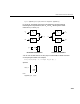
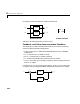

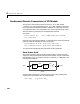
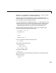
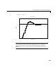
Table Of Contents
- Introduction
- LTI Models
- Operations on LTI Models
- Model Analysis Tools
- Arrays of LTI Models
- Customization
- Setting Toolbox Preferences
- Setting Tool Preferences
- Customizing Response Plot Properties
- Design Case Studies
- Reliable Computations
- GUI Reference
- SISO Design Tool Reference
- Menu Bar
- File
- Import
- Export
- Toolbox Preferences
- Print to Figure
- Close
- Edit
- Undo and Redo
- Root Locus and Bode Diagrams
- SISO Tool Preferences
- View
- Root Locus and Bode Diagrams
- System Data
- Closed Loop Poles
- Design History
- Tools
- Loop Responses
- Continuous/Discrete Conversions
- Draw a Simulink Diagram
- Compensator
- Format
- Edit
- Store
- Retrieve
- Clear
- Window
- Help
- Tool Bar
- Current Compensator
- Feedback Structure
- Root Locus Right-Click Menus
- Bode Diagram Right-Click Menus
- Status Panel
- Menu Bar
- LTI Viewer Reference
- Right-Click Menus for Response Plots
- Function Reference
- Functions by Category
- acker
- allmargin
- append
- augstate
- balreal
- bode
- bodemag
- c2d
- canon
- care
- chgunits
- connect
- covar
- ctrb
- ctrbf
- d2c
- d2d
- damp
- dare
- dcgain
- delay2z
- dlqr
- dlyap
- drss
- dsort
- dss
- dssdata
- esort
- estim
- evalfr
- feedback
- filt
- frd
- frdata
- freqresp
- gensig
- get
- gram
- hasdelay
- impulse
- initial
- interp
- inv
- isct, isdt
- isempty
- isproper
- issiso
- kalman
- kalmd
- lft
- lqgreg
- lqr
- lqrd
- lqry
- lsim
- ltimodels
- ltiprops
- ltiview
- lyap
- margin
- minreal
- modred
- ndims
- ngrid
- nichols
- norm
- nyquist
- obsv
- obsvf
- ord2
- pade
- parallel
- place
- pole
- pzmap
- reg
- reshape
- rlocus
- rss
- series
- set
- sgrid
- sigma
- sisotool
- size
- sminreal
- ss
- ss2ss
- ssbal
- ssdata
- stack
- step
- tf
- tfdata
- totaldelay
- zero
- zgrid
- zpk
- zpkdata
- Index

Continuous/Discrete Conversions of LTI Models
3-21
The signal is then fed to the continuous system , and the resulting
output is sampled every seconds to produce .
Conversely, given a discrete system , the
d2c conversion produces a
continuous system whose ZOH discretization coincides with . This
inverse operation has the following limitations:
•
d2c cannotoperate onLTImodels withpolesat whenthe ZOH isused.
•Negative real poles in the domain are mapped to pairs of complex poles in
the domain. As a result, the
d2c conversion of a discrete system with
negative real poles produces a continuous system with higher order.
The next example illustrates the behavior of
d2c with real negative poles.
Consider the following discrete-time ZPK model.
hd = zpk([],–0.5,1,0.1)
Zero/pole/gain:
1
-------
(z+0.5)
Sampling time: 0.1
Use d2c to convert this model to continuous-time
hc = d2c(hd)
and you get a second-order model.
Zero/pole/gain:
4.621 (s+149.3)
---------------------
(s^2 + 13.86s + 1035)
Discretize the model again
c2d(hc,0.1)
and you get back the original discrete-time system (up to canceling the pole/
zero pair at z=–0.5):
Zero/pole/gain:
(z+0.5)
ut
()
Hs
()
yt
()
T
s
yk
[]
H
d
z
()
Hs
()
H
d
z
()
z 0=
z
s