
Specifications

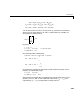
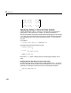
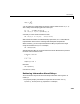

Table Of Contents
- Introduction
- LTI Models
- Operations on LTI Models
- Model Analysis Tools
- Arrays of LTI Models
- Customization
- Setting Toolbox Preferences
- Setting Tool Preferences
- Customizing Response Plot Properties
- Design Case Studies
- Reliable Computations
- GUI Reference
- SISO Design Tool Reference
- Menu Bar
- File
- Import
- Export
- Toolbox Preferences
- Print to Figure
- Close
- Edit
- Undo and Redo
- Root Locus and Bode Diagrams
- SISO Tool Preferences
- View
- Root Locus and Bode Diagrams
- System Data
- Closed Loop Poles
- Design History
- Tools
- Loop Responses
- Continuous/Discrete Conversions
- Draw a Simulink Diagram
- Compensator
- Format
- Edit
- Store
- Retrieve
- Clear
- Window
- Help
- Tool Bar
- Current Compensator
- Feedback Structure
- Root Locus Right-Click Menus
- Bode Diagram Right-Click Menus
- Status Panel
- Menu Bar
- LTI Viewer Reference
- Right-Click Menus for Response Plots
- Function Reference
- Functions by Category
- acker
- allmargin
- append
- augstate
- balreal
- bode
- bodemag
- c2d
- canon
- care
- chgunits
- connect
- covar
- ctrb
- ctrbf
- d2c
- d2d
- damp
- dare
- dcgain
- delay2z
- dlqr
- dlyap
- drss
- dsort
- dss
- dssdata
- esort
- estim
- evalfr
- feedback
- filt
- frd
- frdata
- freqresp
- gensig
- get
- gram
- hasdelay
- impulse
- initial
- interp
- inv
- isct, isdt
- isempty
- isproper
- issiso
- kalman
- kalmd
- lft
- lqgreg
- lqr
- lqrd
- lqry
- lsim
- ltimodels
- ltiprops
- ltiview
- lyap
- margin
- minreal
- modred
- ndims
- ngrid
- nichols
- norm
- nyquist
- obsv
- obsvf
- ord2
- pade
- parallel
- place
- pole
- pzmap
- reg
- reshape
- rlocus
- rss
- series
- set
- sgrid
- sigma
- sisotool
- size
- sminreal
- ss
- ss2ss
- ssbal
- ssdata
- stack
- step
- tf
- tfdata
- totaldelay
- zero
- zgrid
- zpk
- zpkdata
- Index

Time Delays
2-49
You can also use the InputDelay and OutputDelay properties to conveniently
specify input or output delays in TF, ZPK, or FRD models. For example, you
can create the transfer function
by typing
s = tf('s');
H = [1/s ; 2/(s+1)]; % rational part
H.inputdelay = 0.1
The resulting model is displayed as
Transfer function from input to output...
1
#1: exp(–0.1*s) * -
s
2
#2: exp(–0.1*s) * -----
s + 1
By comparison, to produce an equivalent transfer function using the ioDelay
property, you would need to type
H = [1/s ; 2/(s+1)];
H.iodelay = [0.1 ; 0.1];
Notice that the 0.1 second delay is repeated twice in the I/Odelay matrix. More
generally, for a TF, ZPK, or FRD model with input delays and
output delays , the equivalent I/O delay matrix is
x
·
t
()
Ax t
()
B
1
u
1
t 0.1–
()
+ B
2
u
2
t
()
+=
y
1
t 0.2+
()
C
1
xt
()
D
11
u
1
t 0.1–
()
D
12
u
2
t
()
++=
y
2
t 0.3+
()
C
2
xt
()
D
21
u
1
t 0.1–
()
D
22
u
2
t
()
++=
Hs
()
1
s
---
2
s 1+
------------
= e
0.1s–
α
1
... α
m
,,[]
β
1
... β
p
,,[]