
Specifications
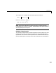
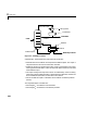

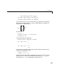
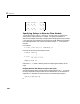
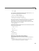

Table Of Contents
- Introduction
- LTI Models
- Operations on LTI Models
- Model Analysis Tools
- Arrays of LTI Models
- Customization
- Setting Toolbox Preferences
- Setting Tool Preferences
- Customizing Response Plot Properties
- Design Case Studies
- Reliable Computations
- GUI Reference
- SISO Design Tool Reference
- Menu Bar
- File
- Import
- Export
- Toolbox Preferences
- Print to Figure
- Close
- Edit
- Undo and Redo
- Root Locus and Bode Diagrams
- SISO Tool Preferences
- View
- Root Locus and Bode Diagrams
- System Data
- Closed Loop Poles
- Design History
- Tools
- Loop Responses
- Continuous/Discrete Conversions
- Draw a Simulink Diagram
- Compensator
- Format
- Edit
- Store
- Retrieve
- Clear
- Window
- Help
- Tool Bar
- Current Compensator
- Feedback Structure
- Root Locus Right-Click Menus
- Bode Diagram Right-Click Menus
- Status Panel
- Menu Bar
- LTI Viewer Reference
- Right-Click Menus for Response Plots
- Function Reference
- Functions by Category
- acker
- allmargin
- append
- augstate
- balreal
- bode
- bodemag
- c2d
- canon
- care
- chgunits
- connect
- covar
- ctrb
- ctrbf
- d2c
- d2d
- damp
- dare
- dcgain
- delay2z
- dlqr
- dlyap
- drss
- dsort
- dss
- dssdata
- esort
- estim
- evalfr
- feedback
- filt
- frd
- frdata
- freqresp
- gensig
- get
- gram
- hasdelay
- impulse
- initial
- interp
- inv
- isct, isdt
- isempty
- isproper
- issiso
- kalman
- kalmd
- lft
- lqgreg
- lqr
- lqrd
- lqry
- lsim
- ltimodels
- ltiprops
- ltiview
- lyap
- margin
- minreal
- modred
- ndims
- ngrid
- nichols
- norm
- nyquist
- obsv
- obsvf
- ord2
- pade
- parallel
- place
- pole
- pzmap
- reg
- reshape
- rlocus
- rss
- series
- set
- sgrid
- sigma
- sisotool
- size
- sminreal
- ss
- ss2ss
- ssbal
- ssdata
- stack
- step
- tf
- tfdata
- totaldelay
- zero
- zgrid
- zpk
- zpkdata
- Index

Time Delays
2-47
Thegoalistomaximize byadjustingtherefluxflowrate andthesteam
flow rate in the reboiler.
To obtain a linearized model around the steady-state operating conditions, the
transient responses to pulses in steam and reflux flow are fitted by first-order
plus delay models. The resulting transfer function model is
Note the different time delays for each input/output pair.
You can specify this MIMO transfer function by typing
H = tf({12.8 –18.9;6.6 –19.4},...
{[16.7 1] [21 1];[10.9 1] [14.4 1]},...
'iodelay',[1 3;7 3],...
'inputname',{'R' , 'S'},...
'outputname',{'Xd' , 'Xb'})
The resulting TF model is displayed as
Transfer function from input "R" to output...
12.8
Xd: exp(–1*s) * ----------
16.7 s + 1
6.6
Xb: exp(–7*s) * ----------
10.9 s + 1
Transfer function from input "S" to output...
–18.9
Xd: exp(–3*s) * --------
21 s + 1
–19.4
Xb: exp(–3*s) * ----------
14.4 s + 1
X
D
R
S
X
D
s
()
X
B
s
()
12.8e
1s–
16.7e 1+
------------------------
18.9e
3s–
–
21.0s 1+
-------------------------
6.6e
7s–
10.9s 1+
------------------------
19.4e
3s–
–
14.4s 1+
-------------------------
Rs
()
Ss
()
=