
Specifications
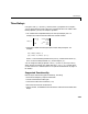
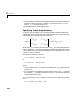
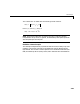

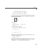
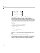

Table Of Contents
- Introduction
- LTI Models
- Operations on LTI Models
- Model Analysis Tools
- Arrays of LTI Models
- Customization
- Setting Toolbox Preferences
- Setting Tool Preferences
- Customizing Response Plot Properties
- Design Case Studies
- Reliable Computations
- GUI Reference
- SISO Design Tool Reference
- Menu Bar
- File
- Import
- Export
- Toolbox Preferences
- Print to Figure
- Close
- Edit
- Undo and Redo
- Root Locus and Bode Diagrams
- SISO Tool Preferences
- View
- Root Locus and Bode Diagrams
- System Data
- Closed Loop Poles
- Design History
- Tools
- Loop Responses
- Continuous/Discrete Conversions
- Draw a Simulink Diagram
- Compensator
- Format
- Edit
- Store
- Retrieve
- Clear
- Window
- Help
- Tool Bar
- Current Compensator
- Feedback Structure
- Root Locus Right-Click Menus
- Bode Diagram Right-Click Menus
- Status Panel
- Menu Bar
- LTI Viewer Reference
- Right-Click Menus for Response Plots
- Function Reference
- Functions by Category
- acker
- allmargin
- append
- augstate
- balreal
- bode
- bodemag
- c2d
- canon
- care
- chgunits
- connect
- covar
- ctrb
- ctrbf
- d2c
- d2d
- damp
- dare
- dcgain
- delay2z
- dlqr
- dlyap
- drss
- dsort
- dss
- dssdata
- esort
- estim
- evalfr
- feedback
- filt
- frd
- frdata
- freqresp
- gensig
- get
- gram
- hasdelay
- impulse
- initial
- interp
- inv
- isct, isdt
- isempty
- isproper
- issiso
- kalman
- kalmd
- lft
- lqgreg
- lqr
- lqrd
- lqry
- lsim
- ltimodels
- ltiprops
- ltiview
- lyap
- margin
- minreal
- modred
- ndims
- ngrid
- nichols
- norm
- nyquist
- obsv
- obsvf
- ord2
- pade
- parallel
- place
- pole
- pzmap
- reg
- reshape
- rlocus
- rss
- series
- set
- sgrid
- sigma
- sisotool
- size
- sminreal
- ss
- ss2ss
- ssbal
- ssdata
- stack
- step
- tf
- tfdata
- totaldelay
- zero
- zgrid
- zpk
- zpkdata
- Index

2 LTI Models
2-44
•Interconnections of continuous-time delay systems as long as the resulting
transfer function from input to output is of the form
where is a rational function of
•Padé approximation of time delays (
pade)
Specifying Input/Output Delays
Using the ioDelay property, you can specify frequency-domain models with
independent delays in each entry of the transfer function. In continuous time,
such models have a transfer function of the form
where the ’s are rational functions of , and is the time delay between
input and output . See “Specifying Delays inDiscrete-Time Models” on page
2-50 for details on the discrete-time counterpart. We collectively refer to the
scalars as the I/O delays.
The syntax to create above is
H = tf(num,den,'ioDelay',Tau)
or
H = zpk(z,p,k,'ioDelay',Tau)
where
•
num, den (respectively,z, p, k) specify the rational part ofthe transfer
function
•
Tau is the matrix of time delays for each I/O pair. That is, Tau(i,j) specifies
the I/O delay in seconds. Note that
Tau and should have the same
row and column dimensions.
You can also use the
ioDelay property in conjunction with state-space models,
as in
sys = ss(A,B,C,D,'ioDelay',Tau)
j
is
τ
ij
–
()
h
ij
s
()
exp
h
ij
s
()
s
Hs
()
e
s
τ
11
–
h
11
s
()
... e
s
τ
1m
–
h
1m
s
()
::
e
s
τ
p1
–
h
p1
s
()
... e
s
τ
pm
–
h
pm
s
()
s
τ
ij
–
()
h
ij
s
()
exp
[]
==
h
ij
s
τ
ij
j
i
τ
ij
Hs
()
h
ij
s
()[]
Hs
()
τ
ij
Hs
()