
Specifications
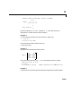
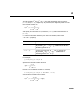


Table Of Contents
- Introduction
- LTI Models
- Operations on LTI Models
- Model Analysis Tools
- Arrays of LTI Models
- Customization
- Setting Toolbox Preferences
- Setting Tool Preferences
- Customizing Response Plot Properties
- Design Case Studies
- Reliable Computations
- GUI Reference
- SISO Design Tool Reference
- Menu Bar
- File
- Import
- Export
- Toolbox Preferences
- Print to Figure
- Close
- Edit
- Undo and Redo
- Root Locus and Bode Diagrams
- SISO Tool Preferences
- View
- Root Locus and Bode Diagrams
- System Data
- Closed Loop Poles
- Design History
- Tools
- Loop Responses
- Continuous/Discrete Conversions
- Draw a Simulink Diagram
- Compensator
- Format
- Edit
- Store
- Retrieve
- Clear
- Window
- Help
- Tool Bar
- Current Compensator
- Feedback Structure
- Root Locus Right-Click Menus
- Bode Diagram Right-Click Menus
- Status Panel
- Menu Bar
- LTI Viewer Reference
- Right-Click Menus for Response Plots
- Function Reference
- Functions by Category
- acker
- allmargin
- append
- augstate
- balreal
- bode
- bodemag
- c2d
- canon
- care
- chgunits
- connect
- covar
- ctrb
- ctrbf
- d2c
- d2d
- damp
- dare
- dcgain
- delay2z
- dlqr
- dlyap
- drss
- dsort
- dss
- dssdata
- esort
- estim
- evalfr
- feedback
- filt
- frd
- frdata
- freqresp
- gensig
- get
- gram
- hasdelay
- impulse
- initial
- interp
- inv
- isct, isdt
- isempty
- isproper
- issiso
- kalman
- kalmd
- lft
- lqgreg
- lqr
- lqrd
- lqry
- lsim
- ltimodels
- ltiprops
- ltiview
- lyap
- margin
- minreal
- modred
- ndims
- ngrid
- nichols
- norm
- nyquist
- obsv
- obsvf
- ord2
- pade
- parallel
- place
- pole
- pzmap
- reg
- reshape
- rlocus
- rss
- series
- set
- sgrid
- sigma
- sisotool
- size
- sminreal
- ss
- ss2ss
- ssbal
- ssdata
- stack
- step
- tf
- tfdata
- totaldelay
- zero
- zgrid
- zpk
- zpkdata
- Index

tf
16-223
The polynomials and are then specified by the row vectors
[1 0 0] and [1 2 3], respectively. By contrast, DSP engineers prefer to write
this transfer function as
and specify its numerator as
1 (instead of [1 0 0]) and its denominator as
[1 2 3].
tf switches convention based on your choice of variable (value of the
'Variable' property).
For example,
g = tf([1 1],[1 2 3],0.1)
specifies the discrete transfer function
because is the default variable. In contrast,
h = tf([1 1],[1 2 3],0.1,'variable','z^-1')
uses the DSP convention and creates
Variable Convention
'z'
(default) Use the row vector [ak ... a1 a0] to specify the
polynomial (coefficients ordered in
descending powers of ).
'z^-1', 'q' Use the row vector [b0 b1 ... bk] to specify the
polynomial (coefficients in
ascending powers of or ).
z
2
z
2
2z 3++
hz
1–
()
1
12z
1–
3z
2–
++
----------------------------------------
=
a
k
z
k
... a
1
za
0
++ +
z
b
0
b
1
z
1–
... b
k
z
k–
+++
z
1–
q
gz
()
z 1+
z
2
2z 3++
----------------------------
=
z
hz
1–
()
1 z
1–
+
12z
1–
3z
2–
++
----------------------------------------
zg z()==