
Specifications
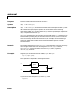
Table Of Contents
- Introduction
- LTI Models
- Operations on LTI Models
- Model Analysis Tools
- Arrays of LTI Models
- Customization
- Setting Toolbox Preferences
- Setting Tool Preferences
- Customizing Response Plot Properties
- Design Case Studies
- Reliable Computations
- GUI Reference
- SISO Design Tool Reference
- Menu Bar
- File
- Import
- Export
- Toolbox Preferences
- Print to Figure
- Close
- Edit
- Undo and Redo
- Root Locus and Bode Diagrams
- SISO Tool Preferences
- View
- Root Locus and Bode Diagrams
- System Data
- Closed Loop Poles
- Design History
- Tools
- Loop Responses
- Continuous/Discrete Conversions
- Draw a Simulink Diagram
- Compensator
- Format
- Edit
- Store
- Retrieve
- Clear
- Window
- Help
- Tool Bar
- Current Compensator
- Feedback Structure
- Root Locus Right-Click Menus
- Bode Diagram Right-Click Menus
- Status Panel
- Menu Bar
- LTI Viewer Reference
- Right-Click Menus for Response Plots
- Function Reference
- Functions by Category
- acker
- allmargin
- append
- augstate
- balreal
- bode
- bodemag
- c2d
- canon
- care
- chgunits
- connect
- covar
- ctrb
- ctrbf
- d2c
- d2d
- damp
- dare
- dcgain
- delay2z
- dlqr
- dlyap
- drss
- dsort
- dss
- dssdata
- esort
- estim
- evalfr
- feedback
- filt
- frd
- frdata
- freqresp
- gensig
- get
- gram
- hasdelay
- impulse
- initial
- interp
- inv
- isct, isdt
- isempty
- isproper
- issiso
- kalman
- kalmd
- lft
- lqgreg
- lqr
- lqrd
- lqry
- lsim
- ltimodels
- ltiprops
- ltiview
- lyap
- margin
- minreal
- modred
- ndims
- ngrid
- nichols
- norm
- nyquist
- obsv
- obsvf
- ord2
- pade
- parallel
- place
- pole
- pzmap
- reg
- reshape
- rlocus
- rss
- series
- set
- sgrid
- sigma
- sisotool
- size
- sminreal
- ss
- ss2ss
- ssbal
- ssdata
- stack
- step
- tf
- tfdata
- totaldelay
- zero
- zgrid
- zpk
- zpkdata
- Index

ss
16-208
sys = ss(A,B,C,D,0.05,'statename',{'position' 'velocity'},...
'inputname','force',...
'notes','Created 10/15/96')
creates a discrete-time model with matrices and sample time 0.05
second. This model has two states labeled
position and velocity,andone
input labeled
force (the dimensions of should be consistent with
these numbers of states and inputs). Finally, a note is attached with the date
ofcreationofthemodel.
Example 2
Compute a state-space realization of the transfer function
by typing
H = [tf([1 1],[1 3 3 2]) ; tf([1 0 3],[1 1 1])];
sys = ss(H);
size(sys)
State-space model with 2 outputs, 1 input, and 5 states.
Note that the number of states is equal to the cumulative order of the SISO
entries of H(s).
To obtain a minimal realization of H(s), type
sys = ss(H,'min');
size(sys)
State-space model with 2 outputs, 1 input, and 3 states.
The resulting state-space model order has order three, the minimum number
of states needed to represent H(s).ThiscanbeseendirectlybyfactoringH(s)
as the product of a first order system with a second order one.
ABCD
,,,
ABCD
,,,
Hs
()
s 1+
s
3
3s
2
3s 2+++
-------------------------------------------
s
2
3+
s
2
s 1++
------------------------
=