
Specifications

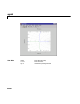
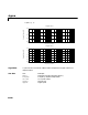
Table Of Contents
- Introduction
- LTI Models
- Operations on LTI Models
- Model Analysis Tools
- Arrays of LTI Models
- Customization
- Setting Toolbox Preferences
- Setting Tool Preferences
- Customizing Response Plot Properties
- Design Case Studies
- Reliable Computations
- GUI Reference
- SISO Design Tool Reference
- Menu Bar
- File
- Import
- Export
- Toolbox Preferences
- Print to Figure
- Close
- Edit
- Undo and Redo
- Root Locus and Bode Diagrams
- SISO Tool Preferences
- View
- Root Locus and Bode Diagrams
- System Data
- Closed Loop Poles
- Design History
- Tools
- Loop Responses
- Continuous/Discrete Conversions
- Draw a Simulink Diagram
- Compensator
- Format
- Edit
- Store
- Retrieve
- Clear
- Window
- Help
- Tool Bar
- Current Compensator
- Feedback Structure
- Root Locus Right-Click Menus
- Bode Diagram Right-Click Menus
- Status Panel
- Menu Bar
- LTI Viewer Reference
- Right-Click Menus for Response Plots
- Function Reference
- Functions by Category
- acker
- allmargin
- append
- augstate
- balreal
- bode
- bodemag
- c2d
- canon
- care
- chgunits
- connect
- covar
- ctrb
- ctrbf
- d2c
- d2d
- damp
- dare
- dcgain
- delay2z
- dlqr
- dlyap
- drss
- dsort
- dss
- dssdata
- esort
- estim
- evalfr
- feedback
- filt
- frd
- frdata
- freqresp
- gensig
- get
- gram
- hasdelay
- impulse
- initial
- interp
- inv
- isct, isdt
- isempty
- isproper
- issiso
- kalman
- kalmd
- lft
- lqgreg
- lqr
- lqrd
- lqry
- lsim
- ltimodels
- ltiprops
- ltiview
- lyap
- margin
- minreal
- modred
- ndims
- ngrid
- nichols
- norm
- nyquist
- obsv
- obsvf
- ord2
- pade
- parallel
- place
- pole
- pzmap
- reg
- reshape
- rlocus
- rss
- series
- set
- sgrid
- sigma
- sisotool
- size
- sminreal
- ss
- ss2ss
- ssbal
- ssdata
- stack
- step
- tf
- tfdata
- totaldelay
- zero
- zgrid
- zpk
- zpkdata
- Index

sigma
16-196
w = {wmin,wmax}. To use particular frequency points, set w to the
corresponding vector of frequencies. Use
logspace to generate logarithmically
spaced frequency vectors. The frequencies must be specified in rad/sec.
sigma(sys,[],type) or sigma(sys,w,type) plots the following modified
singular value responses:
These options are available only for square systems, that is, with the same
number of inputs and outputs.
To superimpose the singular value plots of several LTI models on a single
figure, use
sigma(sys1,sys2,...,sysN)
sigma(sys1,sys2,...,sysN,[],type) % modified SV plot
sigma(sys1,sys2,...,sysN,w) % specify frequency range/grid
The models sys1,sys2,...,sysN need not have the same number of inputs
andoutputs.Eachmodelcanbeeithercontinuous-ordiscrete-time.Youcan
also specify a distinctive color, linestyle, and/or marker for each system plot
with the syntax
sigma(sys1,'PlotStyle1',...,sysN,'PlotStyleN')
See bode for an example.
When invoked with output arguments,
[sv,w] = sigma(sys)
sv = sigma(sys,w)
return the singular values sv of the frequency response at the frequencies w.
For a system with
Nu input and Ny outputs, the array sv has min(Nu,Ny) rows
and as many columns as frequency points (length of
w). The singular values at
the frequency
w(k) are given by sv(:,k).
type = 1
Singular values of the frequency response , where is
the frequency response of
sys.
type = 2
Singular values of the frequency response .
type = 3
Singular values of the frequency response .
H
1–
H
IH+
IH
1–
+