
Specifications
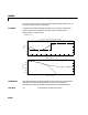
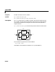
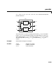
Table Of Contents
- Introduction
- LTI Models
- Operations on LTI Models
- Model Analysis Tools
- Arrays of LTI Models
- Customization
- Setting Toolbox Preferences
- Setting Tool Preferences
- Customizing Response Plot Properties
- Design Case Studies
- Reliable Computations
- GUI Reference
- SISO Design Tool Reference
- Menu Bar
- File
- Import
- Export
- Toolbox Preferences
- Print to Figure
- Close
- Edit
- Undo and Redo
- Root Locus and Bode Diagrams
- SISO Tool Preferences
- View
- Root Locus and Bode Diagrams
- System Data
- Closed Loop Poles
- Design History
- Tools
- Loop Responses
- Continuous/Discrete Conversions
- Draw a Simulink Diagram
- Compensator
- Format
- Edit
- Store
- Retrieve
- Clear
- Window
- Help
- Tool Bar
- Current Compensator
- Feedback Structure
- Root Locus Right-Click Menus
- Bode Diagram Right-Click Menus
- Status Panel
- Menu Bar
- LTI Viewer Reference
- Right-Click Menus for Response Plots
- Function Reference
- Functions by Category
- acker
- allmargin
- append
- augstate
- balreal
- bode
- bodemag
- c2d
- canon
- care
- chgunits
- connect
- covar
- ctrb
- ctrbf
- d2c
- d2d
- damp
- dare
- dcgain
- delay2z
- dlqr
- dlyap
- drss
- dsort
- dss
- dssdata
- esort
- estim
- evalfr
- feedback
- filt
- frd
- frdata
- freqresp
- gensig
- get
- gram
- hasdelay
- impulse
- initial
- interp
- inv
- isct, isdt
- isempty
- isproper
- issiso
- kalman
- kalmd
- lft
- lqgreg
- lqr
- lqrd
- lqry
- lsim
- ltimodels
- ltiprops
- ltiview
- lyap
- margin
- minreal
- modred
- ndims
- ngrid
- nichols
- norm
- nyquist
- obsv
- obsvf
- ord2
- pade
- parallel
- place
- pole
- pzmap
- reg
- reshape
- rlocus
- rss
- series
- set
- sgrid
- sigma
- sisotool
- size
- sminreal
- ss
- ss2ss
- ssbal
- ssdata
- stack
- step
- tf
- tfdata
- totaldelay
- zero
- zgrid
- zpk
- zpkdata
- Index

pade
16-165
16pade
Purpose Compute the Padé approximation of models with time delays
Syntax [num,den] = pade(T,N)
pade(T,N)
sysx = pade(sys,N)
sysx = pade(sys,NI,NO,Nio)
Description pade approximates time delays by rational LTI models. Such approximations
are useful to model time delay effects such as transport and computation
delays within the context of continuous-time systems. The Laplace transform
of an time delay of seconds is . This exponential transfer function
is approximated by a rational transfer function using the Padé approximation
formulas [1].
[num,den] = pade(T,N) returns the Nth-order(diagonal) Padéapproximation
of the continuous-time I/O delay in transfer function form. The row
vectors
num and den contain the numerator and denominator coefficients in
descending powers of . Both are
Nth-order polynomials.
When invoked without output arguments,
pade(T,N)
plots the step and phase responses of the Nth-order Padé approximation and
compares them with the exact responses of the model with I/O delay
T.Note
that the Padé approximation has unit gain at all frequencies.
sysx = pade(sys,N) produces a delay-free approximation sysx of the
continuous delay system
sys. All delays are replaced by their Nth-order Padé
approximation. See Time Delays for details on LTI models with delays.
sysx = pade(sys,NI,NO,Nio) specifies independent approximation orders for
each input, output, and I/O delay. These approximation orders are given by the
arrays of integers
NI, NO,andNio,suchthat:
•
NI(j) is the approximation order for the j-th input channel.
•
NO(i) is the approximation order for the i-th output channel.
•
Nio(i,j) is the approximationorderfor the I/O delay from input j to output
i.
TsT–
()
exp
sT–
()
exp
s