
Specifications
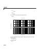
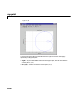
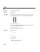
Table Of Contents
- Introduction
- LTI Models
- Operations on LTI Models
- Model Analysis Tools
- Arrays of LTI Models
- Customization
- Setting Toolbox Preferences
- Setting Tool Preferences
- Customizing Response Plot Properties
- Design Case Studies
- Reliable Computations
- GUI Reference
- SISO Design Tool Reference
- Menu Bar
- File
- Import
- Export
- Toolbox Preferences
- Print to Figure
- Close
- Edit
- Undo and Redo
- Root Locus and Bode Diagrams
- SISO Tool Preferences
- View
- Root Locus and Bode Diagrams
- System Data
- Closed Loop Poles
- Design History
- Tools
- Loop Responses
- Continuous/Discrete Conversions
- Draw a Simulink Diagram
- Compensator
- Format
- Edit
- Store
- Retrieve
- Clear
- Window
- Help
- Tool Bar
- Current Compensator
- Feedback Structure
- Root Locus Right-Click Menus
- Bode Diagram Right-Click Menus
- Status Panel
- Menu Bar
- LTI Viewer Reference
- Right-Click Menus for Response Plots
- Function Reference
- Functions by Category
- acker
- allmargin
- append
- augstate
- balreal
- bode
- bodemag
- c2d
- canon
- care
- chgunits
- connect
- covar
- ctrb
- ctrbf
- d2c
- d2d
- damp
- dare
- dcgain
- delay2z
- dlqr
- dlyap
- drss
- dsort
- dss
- dssdata
- esort
- estim
- evalfr
- feedback
- filt
- frd
- frdata
- freqresp
- gensig
- get
- gram
- hasdelay
- impulse
- initial
- interp
- inv
- isct, isdt
- isempty
- isproper
- issiso
- kalman
- kalmd
- lft
- lqgreg
- lqr
- lqrd
- lqry
- lsim
- ltimodels
- ltiprops
- ltiview
- lyap
- margin
- minreal
- modred
- ndims
- ngrid
- nichols
- norm
- nyquist
- obsv
- obsvf
- ord2
- pade
- parallel
- place
- pole
- pzmap
- reg
- reshape
- rlocus
- rss
- series
- set
- sgrid
- sigma
- sisotool
- size
- sminreal
- ss
- ss2ss
- ssbal
- ssdata
- stack
- step
- tf
- tfdata
- totaldelay
- zero
- zgrid
- zpk
- zpkdata
- Index

nyquist
16-157
[re,im,w] = nyquist(sys)
[re,im] = nyquist(sys,w)
return the real and imaginary parts of the frequency response at the
frequencies
w (in rad/sec). re and im are 3-D arrays with the frequency as last
dimension (see “Arguments” below for details).
Arguments The output arguments re and im are 3-D arrays with dimensions
For SISO systems, the scalars
re(1,1,k) and im(1,1,k) are the real and
imaginary parts of the response at the frequency .
For MIMO systems with transfer function ,
re(:,:,k) and im(:,:,k)
give the real and imaginary parts of (both arrays with as many rows
as outputs and as many columns as inputs). Thus,
where is the transfer function from input to output .
Example Plot the Nyquist response of the system
H = tf([2 5 1],[1 2 3])
number of outputs
()
number of inputs
()×
length of w()×
ω
k
w(k)=
re(1,1,k) Re hj
ω
k
()()
=
im(1,1,k) Im hj
ω
k
()()
=
Hs
()
Hj
ω
k
()
re(i,j,k) Re h
ij
j
ω
k
()()
=
im(i,j,k) Im h
ij
j
ω
k
()()
=
h
ij
j
i
Hs
()
2s
2
5s 1++
s
2
2s 3++
-------------------------------
=