Specifications

lsim
16-127
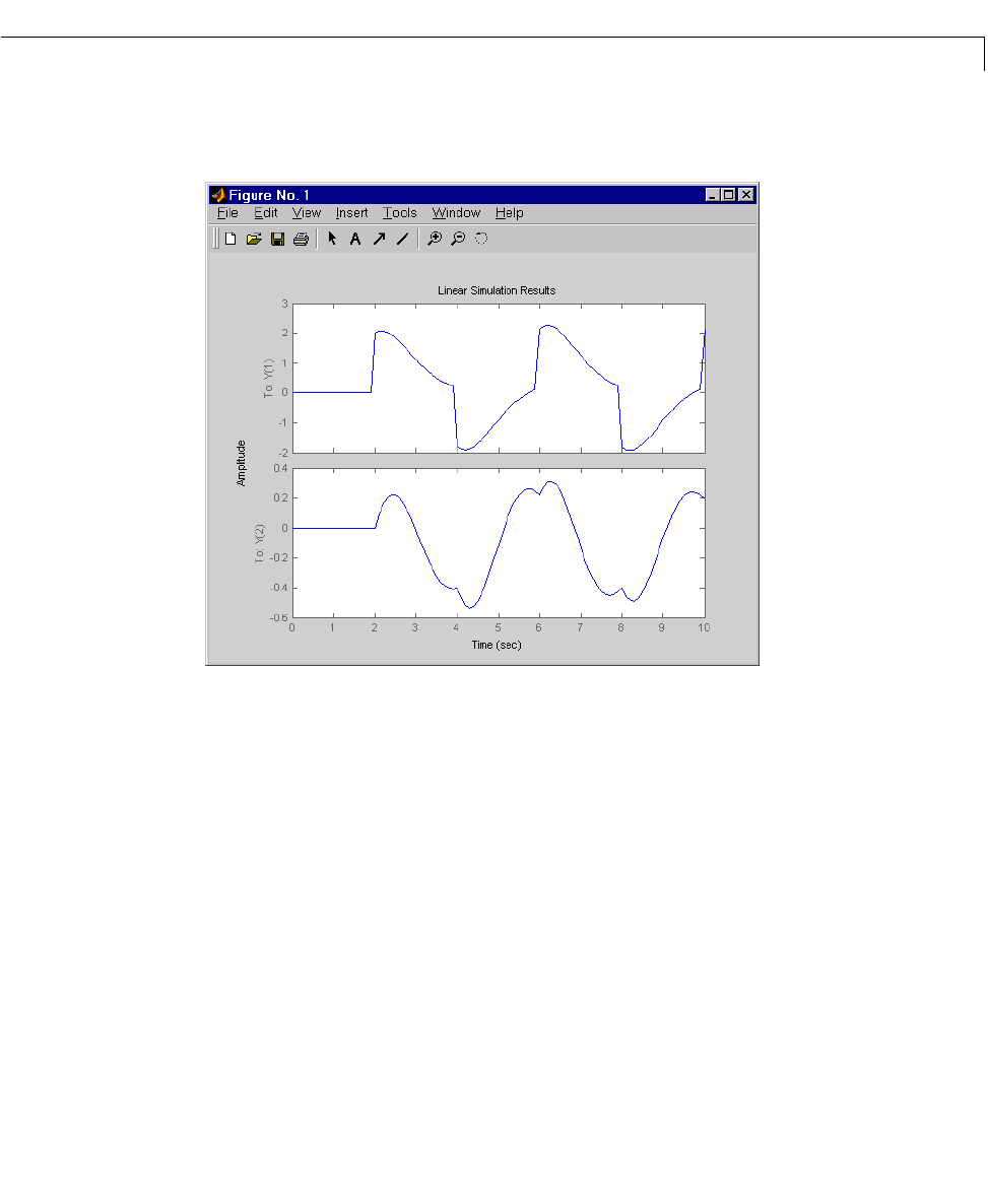
H = [tf([2 5 1],[1 2 3]) ; tf([1 -1],[1 1 5])]
lsim(H,u,t)
Algorithm Discrete-time systems are simulated with ltitr (state space) or filter
(transfer function and zero-pole-gain).
Continuous-time systems are discretized with
c2d using either the 'zoh' or
'foh' method ('foh' is used for smooth input signals and 'zoh' for
discontinuous signals such as pulses or square waves). The sampling period is
set to the spacing
dt between the user-supplied time samples t.
The choice of sampling period can drastically affect simulation results. To
illustrate why, consider the second-order model
Tosimulateitsresponse toasquare wave with period 1second,youcan proceed
as follows:
Hs()
ω
2
s
2
2s ω
2
++
-------------------------------
,= ω 62.83=