
Specifications

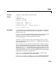
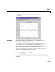


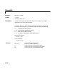
Table Of Contents
- Introduction
- LTI Models
- Operations on LTI Models
- Model Analysis Tools
- Arrays of LTI Models
- Customization
- Setting Toolbox Preferences
- Setting Tool Preferences
- Customizing Response Plot Properties
- Design Case Studies
- Reliable Computations
- GUI Reference
- SISO Design Tool Reference
- Menu Bar
- File
- Import
- Export
- Toolbox Preferences
- Print to Figure
- Close
- Edit
- Undo and Redo
- Root Locus and Bode Diagrams
- SISO Tool Preferences
- View
- Root Locus and Bode Diagrams
- System Data
- Closed Loop Poles
- Design History
- Tools
- Loop Responses
- Continuous/Discrete Conversions
- Draw a Simulink Diagram
- Compensator
- Format
- Edit
- Store
- Retrieve
- Clear
- Window
- Help
- Tool Bar
- Current Compensator
- Feedback Structure
- Root Locus Right-Click Menus
- Bode Diagram Right-Click Menus
- Status Panel
- Menu Bar
- LTI Viewer Reference
- Right-Click Menus for Response Plots
- Function Reference
- Functions by Category
- acker
- allmargin
- append
- augstate
- balreal
- bode
- bodemag
- c2d
- canon
- care
- chgunits
- connect
- covar
- ctrb
- ctrbf
- d2c
- d2d
- damp
- dare
- dcgain
- delay2z
- dlqr
- dlyap
- drss
- dsort
- dss
- dssdata
- esort
- estim
- evalfr
- feedback
- filt
- frd
- frdata
- freqresp
- gensig
- get
- gram
- hasdelay
- impulse
- initial
- interp
- inv
- isct, isdt
- isempty
- isproper
- issiso
- kalman
- kalmd
- lft
- lqgreg
- lqr
- lqrd
- lqry
- lsim
- ltimodels
- ltiprops
- ltiview
- lyap
- margin
- minreal
- modred
- ndims
- ngrid
- nichols
- norm
- nyquist
- obsv
- obsvf
- ord2
- pade
- parallel
- place
- pole
- pzmap
- reg
- reshape
- rlocus
- rss
- series
- set
- sgrid
- sigma
- sisotool
- size
- sminreal
- ss
- ss2ss
- ssbal
- ssdata
- stack
- step
- tf
- tfdata
- totaldelay
- zero
- zgrid
- zpk
- zpkdata
- Index

lsim
16-126
linear interpolation). By default, lsim selects the interpolation method
automatically based on the smoothness of the signal U.
Finally,
lsim(sys1,sys2,...,sysN,u,t)
simulatestheresponsesofseveral LTImodelstothesame inputhistoryt,u and
plots these responses on a single figure. As with
bode or plot, you can specify
a particular color, linestyle, and/or marker for each system, for example,
lsim(sys1,'y:',sys2,'g--',u,t,x0)
The multisystem behavior is similar to that of bode or step.
When invoked with left-hand arguments,
[y,t] = lsim(sys,u,t)
[y,t,x] = lsim(sys,u,t) % for state-space models only
[y,t,x] = lsim(sys,u,t,x0) % with initial state
return the output response y, the time vector t used for simulation, and the
state trajectories
x (for state-space models only). No plot is drawn on the
screen. The matrix
y hasasmanyrowsastimesamples(length(t))andas
many columnsassystemoutputs. Thesameholdsfor
x with “outputs” replaced
bystates. Notethattheoutput
t maydifferfromthe specifiedtimevectorwhen
the input data is undersampled (see “Algorithm”).
Example Simulate and plot the response of the system
to a square wave with period of four seconds. First generate the square wave
with
gensig. Sample every 0.1 second during 10 seconds:
[u,t] = gensig('square',4,10,0.1);
Then simulate with lsim.
Hs
()
2s
2
5s 1++
s
2
2s 3++
-------------------------------
s 1–
s
2
s 5++
------------------------
=