
Specifications

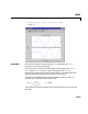


Table Of Contents
- Introduction
- LTI Models
- Operations on LTI Models
- Model Analysis Tools
- Arrays of LTI Models
- Customization
- Setting Toolbox Preferences
- Setting Tool Preferences
- Customizing Response Plot Properties
- Design Case Studies
- Reliable Computations
- GUI Reference
- SISO Design Tool Reference
- Menu Bar
- File
- Import
- Export
- Toolbox Preferences
- Print to Figure
- Close
- Edit
- Undo and Redo
- Root Locus and Bode Diagrams
- SISO Tool Preferences
- View
- Root Locus and Bode Diagrams
- System Data
- Closed Loop Poles
- Design History
- Tools
- Loop Responses
- Continuous/Discrete Conversions
- Draw a Simulink Diagram
- Compensator
- Format
- Edit
- Store
- Retrieve
- Clear
- Window
- Help
- Tool Bar
- Current Compensator
- Feedback Structure
- Root Locus Right-Click Menus
- Bode Diagram Right-Click Menus
- Status Panel
- Menu Bar
- LTI Viewer Reference
- Right-Click Menus for Response Plots
- Function Reference
- Functions by Category
- acker
- allmargin
- append
- augstate
- balreal
- bode
- bodemag
- c2d
- canon
- care
- chgunits
- connect
- covar
- ctrb
- ctrbf
- d2c
- d2d
- damp
- dare
- dcgain
- delay2z
- dlqr
- dlyap
- drss
- dsort
- dss
- dssdata
- esort
- estim
- evalfr
- feedback
- filt
- frd
- frdata
- freqresp
- gensig
- get
- gram
- hasdelay
- impulse
- initial
- interp
- inv
- isct, isdt
- isempty
- isproper
- issiso
- kalman
- kalmd
- lft
- lqgreg
- lqr
- lqrd
- lqry
- lsim
- ltimodels
- ltiprops
- ltiview
- lyap
- margin
- minreal
- modred
- ndims
- ngrid
- nichols
- norm
- nyquist
- obsv
- obsvf
- ord2
- pade
- parallel
- place
- pole
- pzmap
- reg
- reshape
- rlocus
- rss
- series
- set
- sgrid
- sigma
- sisotool
- size
- sminreal
- ss
- ss2ss
- ssbal
- ssdata
- stack
- step
- tf
- tfdata
- totaldelay
- zero
- zgrid
- zpk
- zpkdata
- Index

lsim
16-125
16lsim
Purpose Simulate LTI model response to arbitrary inputs
Syntax lsim(sys,u,t)
lsim(sys,u,t,x0)
lsim(sys,u,t,x0,'zoh')
lsim(sys,u,t,x0,'foh')
lsim(sys1,sys2,...,sysN,u,t)
lsim(sys1,sys2,...,sysN,u,t,x0)
lsim(sys1,'PlotStyle1',...,sysN,'PlotStyleN',u,t)
[y,t,x] = lsim(sys,u,t,x0)
Description lsim simulates the (time) response of continuous or discrete linear systems to
arbitrary inputs. When invoked without left-hand arguments,
lsim plots the
response on the screen.
lsim(sys,u,t) producesaplot ofthetimeresponse oftheLTImodelsys to the
input time history
t,u.Thevectort specifies the time samples for the
simulation and consists of regularly spaced time samples.
t = 0:dt:Tfinal
The matrix u must have as many rows as time samples (length(t))andas
many columns as system inputs. Each row
u(i,:) specifies the input value(s)
atthetimesample
t(i).
The LTI model
sys can be continuous or discrete, SISO or MIMO. In discrete
time,
u mustbesampledatthesamerateasthesystem(t is then redundant
and can be omitted or set to the empty matrix). In continuous time, the time
sampling
dt=t(2)-t(1) is used to discretize the continuous model. If dt is too
large (undersampling),
lsim issues a warning suggesting that you use a more
appropriate sample time, but will use the specifiedsample time.See Algorithm
on page 116 for a discussion of sample times.
lsim(sys,u,t,x0) further specifies an initial condition x0 for the system
states. This syntax applies only to state-space models.
lsim(sys,u,t,x0,'zoh') or lsim(sys,u,t,x0,'foh') explicitlyspecifies how
the input values should be interpolated between samples (zero-order hold or