
Specifications

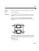
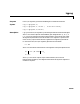
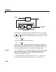
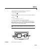

Table Of Contents
- Introduction
- LTI Models
- Operations on LTI Models
- Model Analysis Tools
- Arrays of LTI Models
- Customization
- Setting Toolbox Preferences
- Setting Tool Preferences
- Customizing Response Plot Properties
- Design Case Studies
- Reliable Computations
- GUI Reference
- SISO Design Tool Reference
- Menu Bar
- File
- Import
- Export
- Toolbox Preferences
- Print to Figure
- Close
- Edit
- Undo and Redo
- Root Locus and Bode Diagrams
- SISO Tool Preferences
- View
- Root Locus and Bode Diagrams
- System Data
- Closed Loop Poles
- Design History
- Tools
- Loop Responses
- Continuous/Discrete Conversions
- Draw a Simulink Diagram
- Compensator
- Format
- Edit
- Store
- Retrieve
- Clear
- Window
- Help
- Tool Bar
- Current Compensator
- Feedback Structure
- Root Locus Right-Click Menus
- Bode Diagram Right-Click Menus
- Status Panel
- Menu Bar
- LTI Viewer Reference
- Right-Click Menus for Response Plots
- Function Reference
- Functions by Category
- acker
- allmargin
- append
- augstate
- balreal
- bode
- bodemag
- c2d
- canon
- care
- chgunits
- connect
- covar
- ctrb
- ctrbf
- d2c
- d2d
- damp
- dare
- dcgain
- delay2z
- dlqr
- dlyap
- drss
- dsort
- dss
- dssdata
- esort
- estim
- evalfr
- feedback
- filt
- frd
- frdata
- freqresp
- gensig
- get
- gram
- hasdelay
- impulse
- initial
- interp
- inv
- isct, isdt
- isempty
- isproper
- issiso
- kalman
- kalmd
- lft
- lqgreg
- lqr
- lqrd
- lqry
- lsim
- ltimodels
- ltiprops
- ltiview
- lyap
- margin
- minreal
- modred
- ndims
- ngrid
- nichols
- norm
- nyquist
- obsv
- obsvf
- ord2
- pade
- parallel
- place
- pole
- pzmap
- reg
- reshape
- rlocus
- rss
- series
- set
- sgrid
- sigma
- sisotool
- size
- sminreal
- ss
- ss2ss
- ssbal
- ssdata
- stack
- step
- tf
- tfdata
- totaldelay
- zero
- zgrid
- zpk
- zpkdata
- Index
lqgreg
16-118
In discrete time, you can form the LQG regulator using either the prediction
of basedonmeasurementsup to , or thecurrentstate
estimate based on all available measurements including . While
the regulator
is always well-defined, the current regulator
is causal only when is invertible (see
kalman for the notation). In
addition, practical implementations of the current regulator should allow for
the processing time required to compute once the measurements
become available (this amounts to a time delay in the feedback loop).
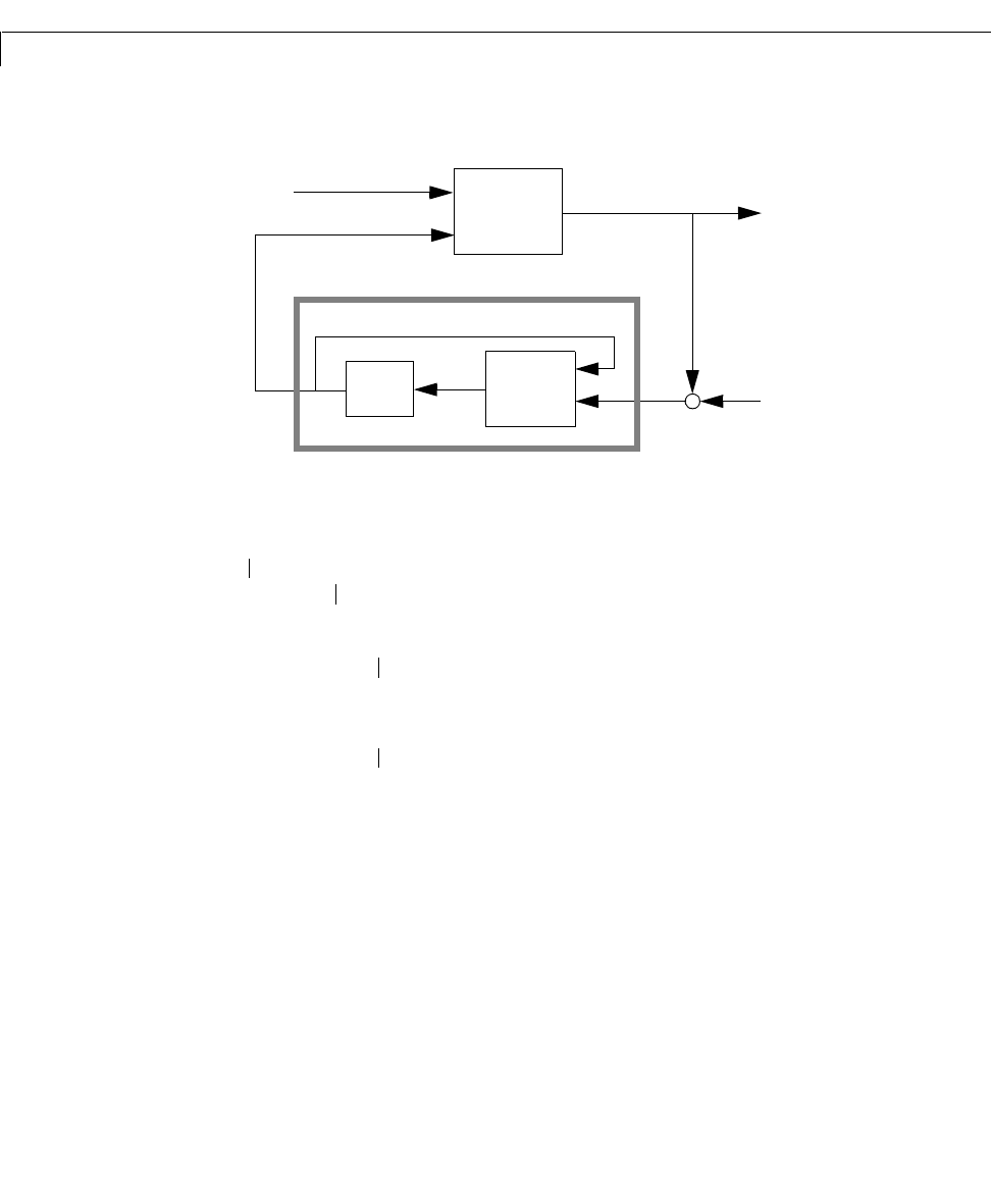
Usage rlqg = lqgreg(kest,k) returns theLQGregulatorrlqg (a state-space model)
given the Kalman estimator
kest and the state-feedback gain matrix k.The
same function handles both continuous- and discrete-time cases. Use
consistent tools to design
kest and k:
• Continuous regulator for continuous plant: use
lqr or lqry and kalman.
• Discrete regulator for discrete plant: use
dlqr or lqry and kalman.
u
y
+
+
x
ˆ
K–
LQG regulator
u
Plant
Measurement
noise
Kalman
filter
Process
noise
y
v
x
ˆ
nn 1–
[]
xn
[]
y
v
n 1–
[]
x
ˆ
nn
[]
y
v
n
[]
un
[]
Kx
ˆ
nn 1–
[]
–=
un
[]
Kx
ˆ
nn
[]
–=
IKMD–
un
[]
y
v
n
[]