
Specifications
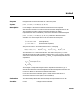

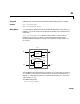
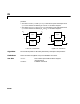
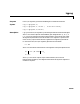
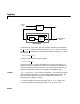
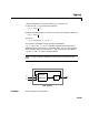
Table Of Contents
- Introduction
- LTI Models
- Operations on LTI Models
- Model Analysis Tools
- Arrays of LTI Models
- Customization
- Setting Toolbox Preferences
- Setting Tool Preferences
- Customizing Response Plot Properties
- Design Case Studies
- Reliable Computations
- GUI Reference
- SISO Design Tool Reference
- Menu Bar
- File
- Import
- Export
- Toolbox Preferences
- Print to Figure
- Close
- Edit
- Undo and Redo
- Root Locus and Bode Diagrams
- SISO Tool Preferences
- View
- Root Locus and Bode Diagrams
- System Data
- Closed Loop Poles
- Design History
- Tools
- Loop Responses
- Continuous/Discrete Conversions
- Draw a Simulink Diagram
- Compensator
- Format
- Edit
- Store
- Retrieve
- Clear
- Window
- Help
- Tool Bar
- Current Compensator
- Feedback Structure
- Root Locus Right-Click Menus
- Bode Diagram Right-Click Menus
- Status Panel
- Menu Bar
- LTI Viewer Reference
- Right-Click Menus for Response Plots
- Function Reference
- Functions by Category
- acker
- allmargin
- append
- augstate
- balreal
- bode
- bodemag
- c2d
- canon
- care
- chgunits
- connect
- covar
- ctrb
- ctrbf
- d2c
- d2d
- damp
- dare
- dcgain
- delay2z
- dlqr
- dlyap
- drss
- dsort
- dss
- dssdata
- esort
- estim
- evalfr
- feedback
- filt
- frd
- frdata
- freqresp
- gensig
- get
- gram
- hasdelay
- impulse
- initial
- interp
- inv
- isct, isdt
- isempty
- isproper
- issiso
- kalman
- kalmd
- lft
- lqgreg
- lqr
- lqrd
- lqry
- lsim
- ltimodels
- ltiprops
- ltiview
- lyap
- margin
- minreal
- modred
- ndims
- ngrid
- nichols
- norm
- nyquist
- obsv
- obsvf
- ord2
- pade
- parallel
- place
- pole
- pzmap
- reg
- reshape
- rlocus
- rss
- series
- set
- sgrid
- sigma
- sisotool
- size
- sminreal
- ss
- ss2ss
- ssbal
- ssdata
- stack
- step
- tf
- tfdata
- totaldelay
- zero
- zgrid
- zpk
- zpkdata
- Index

kalmd
16-113
16kalmd
Purpose Design discrete Kalman estimator for continuous plant
Syntax [kest,L,P,M,Z] = kalmd(sys,Qn,Rn,Ts)
Description kalmd designs a discrete-time Kalman estimator that has response
characteristics similar to a continuous-time estimator designed with
kalman.
This command is useful to derive a discrete estimator for digital
implementation after a satisfactory continuous estimator has been designed.
[kest,L,P,M,Z] = kalmd(sys,Qn,Rn,Ts) produces a discrete Kalman
estimator
kest with sample time Ts for the continuous-time plant
with process noise and measurement noise satisfying
The estimator
kest is derived as follows. The continuous plant sys is first
discretized using zero-order hold with sample time
Ts (see c2d entry), and the
continuous noisecovariancematrices and arereplacedbytheirdiscrete
equivalents
The integral is computed using the matrix exponential formulas in [2]. A
discrete-timeestimator isthendesignedforthediscretizedplantandnoise. See
kalman for details on discrete-time Kalman estimation.
kalmd also returns the estimator gains L and M, and the discrete error
covariance matrices
P and Z (see kalman for details).
Limitations The discretized problem data should satisfy the requirements for kalman.
See Also kalman Design Kalman estimator
x
·
Ax Bu Gw++= (state equation)
y
v
Cx Du v++= (measurement equation)
wv
Ew
()
Ev
()
0, Eww
T
()
Q
n
,= Evv
T
()
R
n
= , Ewv
T
()
0===
Q
n
R
n
Q
d
e
A
τ
GQG
T
e
A
T
τ
τ
d
0
T
s
ò
=
R
d
RT
s
⁄
=