
Specifications
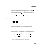

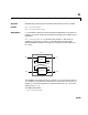
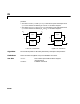
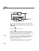
Table Of Contents
- Introduction
- LTI Models
- Operations on LTI Models
- Model Analysis Tools
- Arrays of LTI Models
- Customization
- Setting Toolbox Preferences
- Setting Tool Preferences
- Customizing Response Plot Properties
- Design Case Studies
- Reliable Computations
- GUI Reference
- SISO Design Tool Reference
- Menu Bar
- File
- Import
- Export
- Toolbox Preferences
- Print to Figure
- Close
- Edit
- Undo and Redo
- Root Locus and Bode Diagrams
- SISO Tool Preferences
- View
- Root Locus and Bode Diagrams
- System Data
- Closed Loop Poles
- Design History
- Tools
- Loop Responses
- Continuous/Discrete Conversions
- Draw a Simulink Diagram
- Compensator
- Format
- Edit
- Store
- Retrieve
- Clear
- Window
- Help
- Tool Bar
- Current Compensator
- Feedback Structure
- Root Locus Right-Click Menus
- Bode Diagram Right-Click Menus
- Status Panel
- Menu Bar
- LTI Viewer Reference
- Right-Click Menus for Response Plots
- Function Reference
- Functions by Category
- acker
- allmargin
- append
- augstate
- balreal
- bode
- bodemag
- c2d
- canon
- care
- chgunits
- connect
- covar
- ctrb
- ctrbf
- d2c
- d2d
- damp
- dare
- dcgain
- delay2z
- dlqr
- dlyap
- drss
- dsort
- dss
- dssdata
- esort
- estim
- evalfr
- feedback
- filt
- frd
- frdata
- freqresp
- gensig
- get
- gram
- hasdelay
- impulse
- initial
- interp
- inv
- isct, isdt
- isempty
- isproper
- issiso
- kalman
- kalmd
- lft
- lqgreg
- lqr
- lqrd
- lqry
- lsim
- ltimodels
- ltiprops
- ltiview
- lyap
- margin
- minreal
- modred
- ndims
- ngrid
- nichols
- norm
- nyquist
- obsv
- obsvf
- ord2
- pade
- parallel
- place
- pole
- pzmap
- reg
- reshape
- rlocus
- rss
- series
- set
- sgrid
- sigma
- sisotool
- size
- sminreal
- ss
- ss2ss
- ssbal
- ssdata
- stack
- step
- tf
- tfdata
- totaldelay
- zero
- zgrid
- zpk
- zpkdata
- Index

kalman
16-112
for more general plants sys where the known inputs and stochastic inputs
are mixed together, and not all outputs are measured. The index vectors
sensors and known then specify which outputs of sys are measured and
which inputs are known. All other inputs are assumed stochastic.
Example See LQG Design forthe x-Axis and Kalman Filtering for examples that use the
kalman function.
Limitations The plant and noise data must satisfy:
• detectable
• and
• has no uncontrollable mode on the imaginary
axis (or unit circle in discrete time)
with the notation
See Also care Solve continuous-time Riccati equations
dare Solve discrete-time Riccati equations
estim Form estimator given estimator gain
kalmd Discrete Kalman estimator for continuous plant
lqgreg Assemble LQG regulator
lqr Design state-feedback LQ regulator
References [1]Franklin, G.F.,J.D.Powell, and M.L. Workman, Digital Control of Dynamic
Systems, Second Edition, Addison-Wesley, 1990.
u
w
y
u
CA
,()
R 0
>
QNR
1–
N
T
– 0
≥
ANR
1–
C– QNR
1–
N
T
–
,()
Q GQG
T
=
RRHNN
T
H
T
HQH
T
++ +=
NGQH
T
N+
()
=