
Specifications
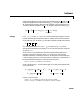

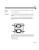
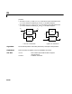
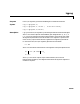
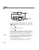
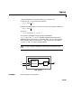

Table Of Contents
- Introduction
- LTI Models
- Operations on LTI Models
- Model Analysis Tools
- Arrays of LTI Models
- Customization
- Setting Toolbox Preferences
- Setting Tool Preferences
- Customizing Response Plot Properties
- Design Case Studies
- Reliable Computations
- GUI Reference
- SISO Design Tool Reference
- Menu Bar
- File
- Import
- Export
- Toolbox Preferences
- Print to Figure
- Close
- Edit
- Undo and Redo
- Root Locus and Bode Diagrams
- SISO Tool Preferences
- View
- Root Locus and Bode Diagrams
- System Data
- Closed Loop Poles
- Design History
- Tools
- Loop Responses
- Continuous/Discrete Conversions
- Draw a Simulink Diagram
- Compensator
- Format
- Edit
- Store
- Retrieve
- Clear
- Window
- Help
- Tool Bar
- Current Compensator
- Feedback Structure
- Root Locus Right-Click Menus
- Bode Diagram Right-Click Menus
- Status Panel
- Menu Bar
- LTI Viewer Reference
- Right-Click Menus for Response Plots
- Function Reference
- Functions by Category
- acker
- allmargin
- append
- augstate
- balreal
- bode
- bodemag
- c2d
- canon
- care
- chgunits
- connect
- covar
- ctrb
- ctrbf
- d2c
- d2d
- damp
- dare
- dcgain
- delay2z
- dlqr
- dlyap
- drss
- dsort
- dss
- dssdata
- esort
- estim
- evalfr
- feedback
- filt
- frd
- frdata
- freqresp
- gensig
- get
- gram
- hasdelay
- impulse
- initial
- interp
- inv
- isct, isdt
- isempty
- isproper
- issiso
- kalman
- kalmd
- lft
- lqgreg
- lqr
- lqrd
- lqry
- lsim
- ltimodels
- ltiprops
- ltiview
- lyap
- margin
- minreal
- modred
- ndims
- ngrid
- nichols
- norm
- nyquist
- obsv
- obsvf
- ord2
- pade
- parallel
- place
- pole
- pzmap
- reg
- reshape
- rlocus
- rss
- series
- set
- sgrid
- sigma
- sisotool
- size
- sminreal
- ss
- ss2ss
- ssbal
- ssdata
- stack
- step
- tf
- tfdata
- totaldelay
- zero
- zgrid
- zpk
- zpkdata
- Index

kalman
16-111
andgeneratesoptimal“current”outputandstateestimates and
using all available measurements including . The gain matrices and
are derived by solving a discrete Riccati equation. The innovation gain
is used to update the prediction using the new measurement .
Usage [kest,L,P] = kalman(sys,Qn,Rn,Nn) returns a state-space model kest of the
Kalman estimator given the plant model
sys and the noise covariance data Qn,
Rn, Nn (matrices above). sys must bea state-space modelwithmatrices
The resulting estimator
kest has as inputs and (or their
discrete-time counterparts) as outputs. You can omit the last input argument
Nn when .
The function
kalman handles both continuous and discrete problems and
produces a continuous estimator when
sys is continuous, and a discrete
estimator otherwise. In continuous time,
kalman also returns the Kalman gain
L and the steady-state error covariance matrix P.NotethatP is the solution of
the associated Riccati equation. In discrete time, the syntax
[kest,L,P,M,Z] = kalman(sys,Qn,Rn,Nn)
returns the filter gain and innovations gain , as well as the steady-state
error covariances
Finally, use the syntaxes
[kest,L,P] = kalman(sys,Qn,Rn,Nn,sensors,known)
[kest,L,P,M,Z] = kalman(sys,Qn,Rn,Nn,sensors,known)
y nn
[]
x nn
[]
y
v
n
[]
L
M M
x
ˆ
nn 1–
[]
y
v
n
[]
x
ˆ
nn
[]
x
ˆ
nn 1–
[]
My
v
n
[]
Cx
ˆ
nn 1–
[]
– Du n
[]
–
()
+=
innovation
ì
QRN
,,
A
BG
C
DH
,,,
uy
v
;
[]
y
ˆ
; x
ˆ
[]
N 0=
LM
PEenn1–
[]
enn 1–
[]
T
()
,
n
∞→
lim= enn 1–
[]
xn
[]
xnn 1–
[]
–=
ZEenn
[]
enn
[]
T
()
,
n
∞→
lim= enn
[]
xn
[]
xnn
[]
–=