
Specifications
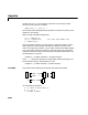
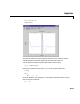
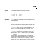
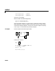
Table Of Contents
- Introduction
- LTI Models
- Operations on LTI Models
- Model Analysis Tools
- Arrays of LTI Models
- Customization
- Setting Toolbox Preferences
- Setting Tool Preferences
- Customizing Response Plot Properties
- Design Case Studies
- Reliable Computations
- GUI Reference
- SISO Design Tool Reference
- Menu Bar
- File
- Import
- Export
- Toolbox Preferences
- Print to Figure
- Close
- Edit
- Undo and Redo
- Root Locus and Bode Diagrams
- SISO Tool Preferences
- View
- Root Locus and Bode Diagrams
- System Data
- Closed Loop Poles
- Design History
- Tools
- Loop Responses
- Continuous/Discrete Conversions
- Draw a Simulink Diagram
- Compensator
- Format
- Edit
- Store
- Retrieve
- Clear
- Window
- Help
- Tool Bar
- Current Compensator
- Feedback Structure
- Root Locus Right-Click Menus
- Bode Diagram Right-Click Menus
- Status Panel
- Menu Bar
- LTI Viewer Reference
- Right-Click Menus for Response Plots
- Function Reference
- Functions by Category
- acker
- allmargin
- append
- augstate
- balreal
- bode
- bodemag
- c2d
- canon
- care
- chgunits
- connect
- covar
- ctrb
- ctrbf
- d2c
- d2d
- damp
- dare
- dcgain
- delay2z
- dlqr
- dlyap
- drss
- dsort
- dss
- dssdata
- esort
- estim
- evalfr
- feedback
- filt
- frd
- frdata
- freqresp
- gensig
- get
- gram
- hasdelay
- impulse
- initial
- interp
- inv
- isct, isdt
- isempty
- isproper
- issiso
- kalman
- kalmd
- lft
- lqgreg
- lqr
- lqrd
- lqry
- lsim
- ltimodels
- ltiprops
- ltiview
- lyap
- margin
- minreal
- modred
- ndims
- ngrid
- nichols
- norm
- nyquist
- obsv
- obsvf
- ord2
- pade
- parallel
- place
- pole
- pzmap
- reg
- reshape
- rlocus
- rss
- series
- set
- sgrid
- sigma
- sisotool
- size
- sminreal
- ss
- ss2ss
- ssbal
- ssdata
- stack
- step
- tf
- tfdata
- totaldelay
- zero
- zgrid
- zpk
- zpkdata
- Index

initial
16-99
16initial
Purpose Compute the initial condition response of state-space models
Syntax initial(sys,x0)
initial(sys,x0,t)
initial(sys1,sys2,...,sysN,x0)
initial(sys1,sys2,...,sysN,x0,t)
initial(sys1,'PlotStyle1',...,sysN,'PlotStyleN',x0)
[y,t,x] = initial(sys,x0)
Description initial calculates the unforcedresponse ofastate-space model with an initial
conditiononthestates.
This function is applicable to either continuous- or discrete-time models. When
invoked without lefthand arguments,
initial plots the initial condition
response on the screen.
initial(sys,x0) plots the response of sys to an initial condition x0 on the
states.
sys can be any state-space model (continuous or discrete, SISO or
MIMO, with or without inputs). The duration of simulation is determined
automatically to reflect adequately the response transients.
initial(sys,x0,t) explicitly sets the simulation horizon. You can specify
either a final time
t = Tfinal (in seconds), or a vector of evenly spaced time
samples of the form
t = 0:dt:Tfinal
For discrete systems, the spacing dt should match the sample period. For
continuous systems,
dt becomes the sample time of the discretized simulation
model (see
impulse), so make sure to choose dt small enough to capture
transient phenomena.
To plot the initial condition responses of several LTI models on a single figure,
use
x
·
Ax ,= x 0
()
x
0
=
yCx=