
Specifications


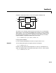


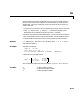
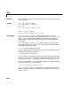
Table Of Contents
- Introduction
- LTI Models
- Operations on LTI Models
- Model Analysis Tools
- Arrays of LTI Models
- Customization
- Setting Toolbox Preferences
- Setting Tool Preferences
- Customizing Response Plot Properties
- Design Case Studies
- Reliable Computations
- GUI Reference
- SISO Design Tool Reference
- Menu Bar
- File
- Import
- Export
- Toolbox Preferences
- Print to Figure
- Close
- Edit
- Undo and Redo
- Root Locus and Bode Diagrams
- SISO Tool Preferences
- View
- Root Locus and Bode Diagrams
- System Data
- Closed Loop Poles
- Design History
- Tools
- Loop Responses
- Continuous/Discrete Conversions
- Draw a Simulink Diagram
- Compensator
- Format
- Edit
- Store
- Retrieve
- Clear
- Window
- Help
- Tool Bar
- Current Compensator
- Feedback Structure
- Root Locus Right-Click Menus
- Bode Diagram Right-Click Menus
- Status Panel
- Menu Bar
- LTI Viewer Reference
- Right-Click Menus for Response Plots
- Function Reference
- Functions by Category
- acker
- allmargin
- append
- augstate
- balreal
- bode
- bodemag
- c2d
- canon
- care
- chgunits
- connect
- covar
- ctrb
- ctrbf
- d2c
- d2d
- damp
- dare
- dcgain
- delay2z
- dlqr
- dlyap
- drss
- dsort
- dss
- dssdata
- esort
- estim
- evalfr
- feedback
- filt
- frd
- frdata
- freqresp
- gensig
- get
- gram
- hasdelay
- impulse
- initial
- interp
- inv
- isct, isdt
- isempty
- isproper
- issiso
- kalman
- kalmd
- lft
- lqgreg
- lqr
- lqrd
- lqry
- lsim
- ltimodels
- ltiprops
- ltiview
- lyap
- margin
- minreal
- modred
- ndims
- ngrid
- nichols
- norm
- nyquist
- obsv
- obsvf
- ord2
- pade
- parallel
- place
- pole
- pzmap
- reg
- reshape
- rlocus
- rss
- series
- set
- sgrid
- sigma
- sisotool
- size
- sminreal
- ss
- ss2ss
- ssbal
- ssdata
- stack
- step
- tf
- tfdata
- totaldelay
- zero
- zgrid
- zpk
- zpkdata
- Index
estim
16-72
estim handles both continuous- and discrete-time cases. You can use the
functions
place (pole placement) or kalman (Kalman filtering) to design an
adequate estimator gain . Note that the estimator poles (eigenvalues of
) should be faster than the plant dynamics (eigenvalues of ) to ensure
accurate estimation.
Example Consider a state-space model sys with sevenoutputs and four inputs. Suppose
you designed a Kalman gain matrix using outputs 4, 7, and 1 of the plant as
sensor measurements, and inputs 1,4, and 3 of the plant as known
(deterministic) inputs. You can then form the Kalman estimator by
sensors = [4,7,1];
known = [1,4,3];
est = estim(sys,L,sensors,known)
See the function kalman for direct Kalman estimator design.
See Also kalman Design Kalman estimator
place Pole placement
reg Form regulator given state-feedback and estimator
gains
x
ˆ
·
Ax
ˆ
B
2
uLyC
2
x
ˆ
D
22
u––
()
++=
y
ˆ
x
ˆ
C
2
I
x
ˆ
D
22
0
u+=
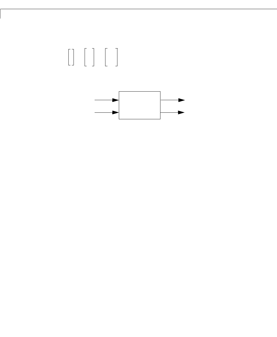
est
u (known)
y (sensors)
y
ˆ
x
ˆ
L
ALC– A
L