
Specifications
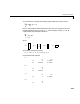


Table Of Contents
- Introduction
- LTI Models
- Operations on LTI Models
- Model Analysis Tools
- Arrays of LTI Models
- Customization
- Setting Toolbox Preferences
- Setting Tool Preferences
- Customizing Response Plot Properties
- Design Case Studies
- Reliable Computations
- GUI Reference
- SISO Design Tool Reference
- Menu Bar
- File
- Import
- Export
- Toolbox Preferences
- Print to Figure
- Close
- Edit
- Undo and Redo
- Root Locus and Bode Diagrams
- SISO Tool Preferences
- View
- Root Locus and Bode Diagrams
- System Data
- Closed Loop Poles
- Design History
- Tools
- Loop Responses
- Continuous/Discrete Conversions
- Draw a Simulink Diagram
- Compensator
- Format
- Edit
- Store
- Retrieve
- Clear
- Window
- Help
- Tool Bar
- Current Compensator
- Feedback Structure
- Root Locus Right-Click Menus
- Bode Diagram Right-Click Menus
- Status Panel
- Menu Bar
- LTI Viewer Reference
- Right-Click Menus for Response Plots
- Function Reference
- Functions by Category
- acker
- allmargin
- append
- augstate
- balreal
- bode
- bodemag
- c2d
- canon
- care
- chgunits
- connect
- covar
- ctrb
- ctrbf
- d2c
- d2d
- damp
- dare
- dcgain
- delay2z
- dlqr
- dlyap
- drss
- dsort
- dss
- dssdata
- esort
- estim
- evalfr
- feedback
- filt
- frd
- frdata
- freqresp
- gensig
- get
- gram
- hasdelay
- impulse
- initial
- interp
- inv
- isct, isdt
- isempty
- isproper
- issiso
- kalman
- kalmd
- lft
- lqgreg
- lqr
- lqrd
- lqry
- lsim
- ltimodels
- ltiprops
- ltiview
- lyap
- margin
- minreal
- modred
- ndims
- ngrid
- nichols
- norm
- nyquist
- obsv
- obsvf
- ord2
- pade
- parallel
- place
- pole
- pzmap
- reg
- reshape
- rlocus
- rss
- series
- set
- sgrid
- sigma
- sisotool
- size
- sminreal
- ss
- ss2ss
- ssbal
- ssdata
- stack
- step
- tf
- tfdata
- totaldelay
- zero
- zgrid
- zpk
- zpkdata
- Index

2 LTI Models
2-22
clashes with the “descending powers of ”conventionassumedbytf (see
“Transfer Function Models” on page 2-8, or
tf). For example,
h = tf([1 0.5],[1 2 3])
produces the transfer function
which differs from by a factor .
Toavoidsuchconventionclashes, theControlSystem Toolboxoffersaseparate
function
filt dedicated to the DSP-like specification of transfer functions. Its
syntax is
h = filt(num,den)
for discrete transfer functions with unspecified sample time, and
h = filt(num,den,Ts)
to further specify the sample time Ts. This function creates TF objects just like
tf,butexpectsnum and den to list the numerator and denominator coefficients
in ascending powers of . For example, typing
h = filt([1 0.5],[1 2 3])
produces
Transfer function:
1 + 0.5 z^–1
-------------------
1 + 2 z^–1 + 3 z^–2
Sampling time: unspecified
You can also use filt tospecifyMIMO transfer functionsin . Just as for tf,
the input arguments
num and den are then cell arrays of row vectors of
appropriate dimensions (see “Transfer Function Models” on page 2-8 for
details). Note that each row vector should comply with the “ascending powers
of ” convention.
z
z 0.5+
z
2
2z 3++
----------------------------
Hz
1–
()
z
z
1–
z
1–
z
1–