
Specifications
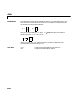
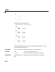

Table Of Contents
- Introduction
- LTI Models
- Operations on LTI Models
- Model Analysis Tools
- Arrays of LTI Models
- Customization
- Setting Toolbox Preferences
- Setting Tool Preferences
- Customizing Response Plot Properties
- Design Case Studies
- Reliable Computations
- GUI Reference
- SISO Design Tool Reference
- Menu Bar
- File
- Import
- Export
- Toolbox Preferences
- Print to Figure
- Close
- Edit
- Undo and Redo
- Root Locus and Bode Diagrams
- SISO Tool Preferences
- View
- Root Locus and Bode Diagrams
- System Data
- Closed Loop Poles
- Design History
- Tools
- Loop Responses
- Continuous/Discrete Conversions
- Draw a Simulink Diagram
- Compensator
- Format
- Edit
- Store
- Retrieve
- Clear
- Window
- Help
- Tool Bar
- Current Compensator
- Feedback Structure
- Root Locus Right-Click Menus
- Bode Diagram Right-Click Menus
- Status Panel
- Menu Bar
- LTI Viewer Reference
- Right-Click Menus for Response Plots
- Function Reference
- Functions by Category
- acker
- allmargin
- append
- augstate
- balreal
- bode
- bodemag
- c2d
- canon
- care
- chgunits
- connect
- covar
- ctrb
- ctrbf
- d2c
- d2d
- damp
- dare
- dcgain
- delay2z
- dlqr
- dlyap
- drss
- dsort
- dss
- dssdata
- esort
- estim
- evalfr
- feedback
- filt
- frd
- frdata
- freqresp
- gensig
- get
- gram
- hasdelay
- impulse
- initial
- interp
- inv
- isct, isdt
- isempty
- isproper
- issiso
- kalman
- kalmd
- lft
- lqgreg
- lqr
- lqrd
- lqry
- lsim
- ltimodels
- ltiprops
- ltiview
- lyap
- margin
- minreal
- modred
- ndims
- ngrid
- nichols
- norm
- nyquist
- obsv
- obsvf
- ord2
- pade
- parallel
- place
- pole
- pzmap
- reg
- reshape
- rlocus
- rss
- series
- set
- sgrid
- sigma
- sisotool
- size
- sminreal
- ss
- ss2ss
- ssbal
- ssdata
- stack
- step
- tf
- tfdata
- totaldelay
- zero
- zgrid
- zpk
- zpkdata
- Index

d2c
16-50
c2d(Hc,0.1,'tustin')
gives back the original .
Algorithm The 'zoh' conversion is performed in state space and relies on the matrix
logarithm (see
logm in Using MATLAB).
Limitations The Tustin approximation is not defined for systems with poles at and
is ill-conditioned for systems with poles near .
The zero-order hold method cannot handle systems with poles at . In
addition, the
'zoh' conversion increases the model order for systems with
negative real poles, [2]. This is necessary because the matrix logarithm maps
real negative poles to complexpoles. As a result, a discrete model with asingle
pole at would be transformed to a continuous model with a single
complex pole at . Such a model is not meaningful
because of its complex time response.
To ensure that all complex poles of the continuous model come in conjugate
pairs,
d2c replaces negative real poles withapair of complex conjugate
poles near . The conversion then yields a continuous model with higher
order. For example, the discrete model with transfer function
and sample time 0.1 second is converted by typing
Ts = 0.1
H = zpk(-0.2,-0.5,1,Ts) * tf(1,[1 1 0.4],Ts)
Hc = d2c(H)
MATLAB responds with
Warning: System order was increased to handle real negative poles.
Zero/pole/gain:
-33.6556 (s-6.273) (s^2 + 28.29s + 1041)
--------------------------------------------
(s^2 + 9.163s + 637.3) (s^2 + 13.86s + 1035)
Convert Hc back to discrete time by typing
Hz
()
z 1–=
z 1–=
z 0=
z 0.5–=
0.5–
()
log 0.6931– j
π
+
≈
z
α
–=
α
–
Hz
()
z 0.2+
z 0.5+
()
z
2
z 0.4++
()
---------------------------------------------------------
=