Specifications

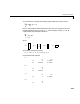
Table Of Contents

Creating LTI Models

2-21

creates the same TF model as

H = tf([1 2], [1 0.6 0.9], 0.1);

Similarly,

z = zpk('z', 0.1);

H = [z/(z+0.1)/(z+0.2) ; (z^2+0.2*z+0.1)/(z^2+0.2*z+0.01)]

produces the single-input, two-output ZPK model

Zero/pole/gain from input to output...

#1: ---------------

(z+0.1) (z+0.2)

(z^2 + 0.2z + 0.1)

#2: ------------------

(z+0.1)^2

Sampling time: 0.1

Note that:

•The syntax

z = tf('z') is equivalent to z = tf('z',–1) and leaves the

sample time unspecified. The same applies to

z = zpk('z').

•Once you have defined

z as indicated above, any rational expressions in z

createsadiscrete-timemodelofthesametypeandwiththesamesample

time as

Discrete Transfer Functions in DSP Format

In digital signal processing (DSP), it is customary to write discrete transfer

functions as rational expressions in and to order the numerator and

denominator coefficients in ascending powers of . For example, the

numerator and denominator of

wouldbespecifiedastherowvectors

[1 0.5] and [1 2 3], respectively. When

the numerator and denominator have different degrees, this convention

1–

–

1–

()

10.5z

1–

12z

1–

2–

----------------------------------------