
Specifications
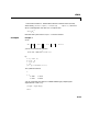

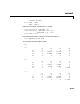
Table Of Contents
- Introduction
- LTI Models
- Operations on LTI Models
- Model Analysis Tools
- Arrays of LTI Models
- Customization
- Setting Toolbox Preferences
- Setting Tool Preferences
- Customizing Response Plot Properties
- Design Case Studies
- Reliable Computations
- GUI Reference
- SISO Design Tool Reference
- Menu Bar
- File
- Import
- Export
- Toolbox Preferences
- Print to Figure
- Close
- Edit
- Undo and Redo
- Root Locus and Bode Diagrams
- SISO Tool Preferences
- View
- Root Locus and Bode Diagrams
- System Data
- Closed Loop Poles
- Design History
- Tools
- Loop Responses
- Continuous/Discrete Conversions
- Draw a Simulink Diagram
- Compensator
- Format
- Edit
- Store
- Retrieve
- Clear
- Window
- Help
- Tool Bar
- Current Compensator
- Feedback Structure
- Root Locus Right-Click Menus
- Bode Diagram Right-Click Menus
- Status Panel
- Menu Bar
- LTI Viewer Reference
- Right-Click Menus for Response Plots
- Function Reference
- Functions by Category
- acker
- allmargin
- append
- augstate
- balreal
- bode
- bodemag
- c2d
- canon
- care
- chgunits
- connect
- covar
- ctrb
- ctrbf
- d2c
- d2d
- damp
- dare
- dcgain
- delay2z
- dlqr
- dlyap
- drss
- dsort
- dss
- dssdata
- esort
- estim
- evalfr
- feedback
- filt
- frd
- frdata
- freqresp
- gensig
- get
- gram
- hasdelay
- impulse
- initial
- interp
- inv
- isct, isdt
- isempty
- isproper
- issiso
- kalman
- kalmd
- lft
- lqgreg
- lqr
- lqrd
- lqry
- lsim
- ltimodels
- ltiprops
- ltiview
- lyap
- margin
- minreal
- modred
- ndims
- ngrid
- nichols
- norm
- nyquist
- obsv
- obsvf
- ord2
- pade
- parallel
- place
- pole
- pzmap
- reg
- reshape
- rlocus
- rss
- series
- set
- sgrid
- sigma
- sisotool
- size
- sminreal
- ss
- ss2ss
- ssbal
- ssdata
- stack
- step
- tf
- tfdata
- totaldelay
- zero
- zgrid
- zpk
- zpkdata
- Index

connect
16-40
d =
uc u1 u2 ?
? 0 0 0 0
y1 0 -0.5476 -0.141 0
y2 0 -0.6459 0.2958 0
? 0 0 0 2
Continuous-time system.
Note that the ordering of the inputs and outputs is the same as the block
ordering you chose. Unnamed inputs or outputs are denoted by
?.
To derive the overall block diagram model from
sys, specify the
interconnections and the external inputs and outputs. You need to connect
outputs 1 and 4 into input 3 (
u2), and output 3 (y2) into input 4. The
interconnection matrix
Q is therefore
Q = [3 1 -4
4 3 0];
Note that the second row of Q has been padded with a trailing zero. The block
diagram has two external inputs
uc and u1 (inputs 1 and 2 of sys), and two
external outputs
y1 and y2 (outputs 2 and 3 of sys). Accordingly, set inputs
and outputs as follows.
inputs = [1 2];
outputs = [2 3];
You can obtain a state-space model for the overall interconnection by typing
sysc = connect(sys,Q,inputs,outputs)
a =
x1 x2 x3 x4
x1 -5 0 0 0
x2 0.84223 0.076636 5.6007 0.47644
x3 -2.9012 -33.029 45.164 -1.6411
x4 0.65708 -11.996 16.06 -1.6283
b =