
Specifications
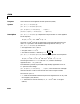
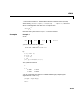

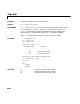

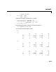
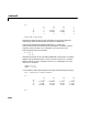
Table Of Contents
- Introduction
- LTI Models
- Operations on LTI Models
- Model Analysis Tools
- Arrays of LTI Models
- Customization
- Setting Toolbox Preferences
- Setting Tool Preferences
- Customizing Response Plot Properties
- Design Case Studies
- Reliable Computations
- GUI Reference
- SISO Design Tool Reference
- Menu Bar
- File
- Import
- Export
- Toolbox Preferences
- Print to Figure
- Close
- Edit
- Undo and Redo
- Root Locus and Bode Diagrams
- SISO Tool Preferences
- View
- Root Locus and Bode Diagrams
- System Data
- Closed Loop Poles
- Design History
- Tools
- Loop Responses
- Continuous/Discrete Conversions
- Draw a Simulink Diagram
- Compensator
- Format
- Edit
- Store
- Retrieve
- Clear
- Window
- Help
- Tool Bar
- Current Compensator
- Feedback Structure
- Root Locus Right-Click Menus
- Bode Diagram Right-Click Menus
- Status Panel
- Menu Bar
- LTI Viewer Reference
- Right-Click Menus for Response Plots
- Function Reference
- Functions by Category
- acker
- allmargin
- append
- augstate
- balreal
- bode
- bodemag
- c2d
- canon
- care
- chgunits
- connect
- covar
- ctrb
- ctrbf
- d2c
- d2d
- damp
- dare
- dcgain
- delay2z
- dlqr
- dlyap
- drss
- dsort
- dss
- dssdata
- esort
- estim
- evalfr
- feedback
- filt
- frd
- frdata
- freqresp
- gensig
- get
- gram
- hasdelay
- impulse
- initial
- interp
- inv
- isct, isdt
- isempty
- isproper
- issiso
- kalman
- kalmd
- lft
- lqgreg
- lqr
- lqrd
- lqry
- lsim
- ltimodels
- ltiprops
- ltiview
- lyap
- margin
- minreal
- modred
- ndims
- ngrid
- nichols
- norm
- nyquist
- obsv
- obsvf
- ord2
- pade
- parallel
- place
- pole
- pzmap
- reg
- reshape
- rlocus
- rss
- series
- set
- sgrid
- sigma
- sisotool
- size
- sminreal
- ss
- ss2ss
- ssbal
- ssdata
- stack
- step
- tf
- tfdata
- totaldelay
- zero
- zgrid
- zpk
- zpkdata
- Index

care
16-34
-3.4495 -3.5026
1.4495 -1.4370
Finally, note that the variable l contains the closed-loop eigenvalues
eig(a-b*g).
l
l =
-3.5026
-1.4370
Example 2
To solve the -like Riccati equation
rewrite it in the
care format as
You can now compute the stabilizing solution by
B = [B1 , B2]
m1 = size(B1,2)
m2 = size(B2,2)
R = [-g^2*eye(m1) zeros(m1,m2) ; zeros(m2,m1) eye(m2)]
X = care(A,B,C'*C,R)
Algorithm care implements the algorithms described in [1]. It works with the
Hamiltonian matrix when is well-conditioned and ; otherwise it uses
the extended Hamiltonian pencil and QZ algorithm.
Limitations The pair must be stabilizable (that is, all unstable modes are
controllable). In addition, the associated Hamiltonian matrix or pencil must
H
∞
A
T
XXAX
γ
2–
B
1
B
1
T
B
2
B
2
T
–
()
X++ C
T
C+ 0=
A
T
XXAXB
1
B
2
,[]
γ
2–
I– 0
0 I
1–
B
1
T
B
2
T
X– C
T
C++0=
B
R
ì
ì
X
REI=
AB,()