
Specifications
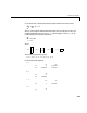


Table Of Contents
- Introduction
- LTI Models
- Operations on LTI Models
- Model Analysis Tools
- Arrays of LTI Models
- Customization
- Setting Toolbox Preferences
- Setting Tool Preferences
- Customizing Response Plot Properties
- Design Case Studies
- Reliable Computations
- GUI Reference
- SISO Design Tool Reference
- Menu Bar
- File
- Import
- Export
- Toolbox Preferences
- Print to Figure
- Close
- Edit
- Undo and Redo
- Root Locus and Bode Diagrams
- SISO Tool Preferences
- View
- Root Locus and Bode Diagrams
- System Data
- Closed Loop Poles
- Design History
- Tools
- Loop Responses
- Continuous/Discrete Conversions
- Draw a Simulink Diagram
- Compensator
- Format
- Edit
- Store
- Retrieve
- Clear
- Window
- Help
- Tool Bar
- Current Compensator
- Feedback Structure
- Root Locus Right-Click Menus
- Bode Diagram Right-Click Menus
- Status Panel
- Menu Bar
- LTI Viewer Reference
- Right-Click Menus for Response Plots
- Function Reference
- Functions by Category
- acker
- allmargin
- append
- augstate
- balreal
- bode
- bodemag
- c2d
- canon
- care
- chgunits
- connect
- covar
- ctrb
- ctrbf
- d2c
- d2d
- damp
- dare
- dcgain
- delay2z
- dlqr
- dlyap
- drss
- dsort
- dss
- dssdata
- esort
- estim
- evalfr
- feedback
- filt
- frd
- frdata
- freqresp
- gensig
- get
- gram
- hasdelay
- impulse
- initial
- interp
- inv
- isct, isdt
- isempty
- isproper
- issiso
- kalman
- kalmd
- lft
- lqgreg
- lqr
- lqrd
- lqry
- lsim
- ltimodels
- ltiprops
- ltiview
- lyap
- margin
- minreal
- modred
- ndims
- ngrid
- nichols
- norm
- nyquist
- obsv
- obsvf
- ord2
- pade
- parallel
- place
- pole
- pzmap
- reg
- reshape
- rlocus
- rss
- series
- set
- sgrid
- sigma
- sisotool
- size
- sminreal
- ss
- ss2ss
- ssbal
- ssdata
- stack
- step
- tf
- tfdata
- totaldelay
- zero
- zgrid
- zpk
- zpkdata
- Index

Creating LTI Models
2-19
Discrete-Time Models
Creating discrete-time models is very much like creating continuous-time
models, except that you must also specify a sampling period or sample time for
discrete-timemodels.Thesampletimevalueshouldbescalarandexpressedin
seconds. You can also use the value –1 to leave the sample time unspecified.
To specify discrete-time LTI models using
tf, zpk, ss,orfrd,simplyappend
the desired sample time value
Ts to the list of inputs.
sys1 = tf(num,den,Ts)
sys2 = zpk(z,p,k,Ts)
sys3 = ss(a,b,c,d,Ts)
sys4 = frd(response,frequency,Ts)
For example,
h = tf([1 –1],[1 –0.5],0.1)
creates the discrete-time transfer function with
sample time 0.1 seconds, and
sys = ss(A,B,C,D,0.5)
specifies the discrete-time state-space model
with sampling period 0.5 second. The vectors denote the
values of the state, input, and output vectors at the nth sample.
MIMO model
with
Ny outputs
and
Nu inputs
Ny-by-Nu-by-Nf multidimensional array for which
response(i,j,k) specifies the frequency response
from input
j to output i at frequency frequency(k)
S1
-by-...-by-Sn
array of models
with
Ny outputs
and
Nu inputs
Ny-by-Nu-by-S1-by-...-by-Sn multidimensional array,
for which
response(i,j,k,:) specifies the array of
frequency response data from input
j to output i at
frequency
frequency(k)
Table 2-3: Data Format for the Argument response in FRD Models (Continued)
Model Form Response Data Format
hz
()
z 1–
()
z 0.5–
()⁄
=
xn 1+[]Ax n[] Bu n[]+=
yn[] Cx n[] Du n[]+=
xn[]un[]yn[],,