Specifications

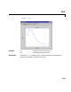
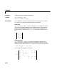
Table Of Contents

bode

16-24

bode(g,'r',gd,'b--')

Algorithm For continuous-time systems, bode computes the frequency response by

evaluating the transfer function on the imaginary axis . Only

positive frequencies are considered. For state-space models, the frequency

response is

When numerically safe, is diagonalized for maximum speed. Otherwise,

is reduced to upper Hessenberg form and the linear equation

is solved at each frequency point, taking advantage of the Hessenberg

structure. The reduction to Hessenberg form provides a good compromise

between efficiency and reliability. See [1] for more details on this technique.

For discrete-time systems, the frequency response is obtained by evaluating

the transfer function on the unit circle. To facilitate interpretation, the

upper-half of the unit circle is parametrized as

()

DCj

A–

()

1–

B+ ,

≥

A–

()

XB=

Hz()

= ,0ωω

≤≤

------