
Specifications

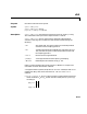
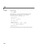
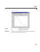
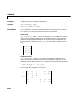
Table Of Contents
- Introduction
- LTI Models
- Operations on LTI Models
- Model Analysis Tools
- Arrays of LTI Models
- Customization
- Setting Toolbox Preferences
- Setting Tool Preferences
- Customizing Response Plot Properties
- Design Case Studies
- Reliable Computations
- GUI Reference
- SISO Design Tool Reference
- Menu Bar
- File
- Import
- Export
- Toolbox Preferences
- Print to Figure
- Close
- Edit
- Undo and Redo
- Root Locus and Bode Diagrams
- SISO Tool Preferences
- View
- Root Locus and Bode Diagrams
- System Data
- Closed Loop Poles
- Design History
- Tools
- Loop Responses
- Continuous/Discrete Conversions
- Draw a Simulink Diagram
- Compensator
- Format
- Edit
- Store
- Retrieve
- Clear
- Window
- Help
- Tool Bar
- Current Compensator
- Feedback Structure
- Root Locus Right-Click Menus
- Bode Diagram Right-Click Menus
- Status Panel
- Menu Bar
- LTI Viewer Reference
- Right-Click Menus for Response Plots
- Function Reference
- Functions by Category
- acker
- allmargin
- append
- augstate
- balreal
- bode
- bodemag
- c2d
- canon
- care
- chgunits
- connect
- covar
- ctrb
- ctrbf
- d2c
- d2d
- damp
- dare
- dcgain
- delay2z
- dlqr
- dlyap
- drss
- dsort
- dss
- dssdata
- esort
- estim
- evalfr
- feedback
- filt
- frd
- frdata
- freqresp
- gensig
- get
- gram
- hasdelay
- impulse
- initial
- interp
- inv
- isct, isdt
- isempty
- isproper
- issiso
- kalman
- kalmd
- lft
- lqgreg
- lqr
- lqrd
- lqry
- lsim
- ltimodels
- ltiprops
- ltiview
- lyap
- margin
- minreal
- modred
- ndims
- ngrid
- nichols
- norm
- nyquist
- obsv
- obsvf
- ord2
- pade
- parallel
- place
- pole
- pzmap
- reg
- reshape
- rlocus
- rss
- series
- set
- sgrid
- sigma
- sisotool
- size
- sminreal
- ss
- ss2ss
- ssbal
- ssdata
- stack
- step
- tf
- tfdata
- totaldelay
- zero
- zgrid
- zpk
- zpkdata
- Index

bode
16-22
uses red dashed lines for the first system sys1 and green 'x' markers for the
second system
sys2.
When invoked with left-hand arguments
[mag,phase,w] = bode(sys)
[mag,phase] = bode(sys,w)
return the magnitude and phase (in degrees) of the frequency response at the
frequencies
w (in rad/sec). The outputs mag and phase are 3-D arrays with the
frequency as the last dimension (see “Arguments” below for details). You can
convert the magnitude to decibels by
magdb = 20*log10(mag)
Remark If sys is an FRD model, bode(sys,w), w can only include frequencies in
sys.frequency.
Arguments The output arguments mag and phase are 3-D arrays with dimensions
For SISO systems,
mag(1,1,k) and phase(1,1,k) give the magnitude and
phase of the response at the frequency =
w(k).
MIMO systems are treated as arrays of SISO systems and the magnitudes and
phases are computed for each SISO entry h
ij
independently (h
ij
is the transfer
function from input j to output i). The values
mag(i,j,k) and phase(i,j,k)
then characterize the response of h
ij
at the frequency w(k).
Example You can plot the Bode response of the continuous SISO system
number of outputs
()
number of inputs
()×
length of
w()×
ω
k
mag(1,1,k) hj
ω
k
()
=
phase(1,1,k) hj
ω
k
()∠
=
mag(i,j,k) h
ij
j
ω
k
()
=
phase(i,j,k) h
ij
j
ω
k
()∠
=