
Specifications
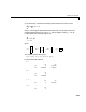
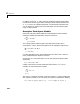
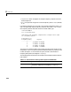


Table Of Contents
- Introduction
- LTI Models
- Operations on LTI Models
- Model Analysis Tools
- Arrays of LTI Models
- Customization
- Setting Toolbox Preferences
- Setting Tool Preferences
- Customizing Response Plot Properties
- Design Case Studies
- Reliable Computations
- GUI Reference
- SISO Design Tool Reference
- Menu Bar
- File
- Import
- Export
- Toolbox Preferences
- Print to Figure
- Close
- Edit
- Undo and Redo
- Root Locus and Bode Diagrams
- SISO Tool Preferences
- View
- Root Locus and Bode Diagrams
- System Data
- Closed Loop Poles
- Design History
- Tools
- Loop Responses
- Continuous/Discrete Conversions
- Draw a Simulink Diagram
- Compensator
- Format
- Edit
- Store
- Retrieve
- Clear
- Window
- Help
- Tool Bar
- Current Compensator
- Feedback Structure
- Root Locus Right-Click Menus
- Bode Diagram Right-Click Menus
- Status Panel
- Menu Bar
- LTI Viewer Reference
- Right-Click Menus for Response Plots
- Function Reference
- Functions by Category
- acker
- allmargin
- append
- augstate
- balreal
- bode
- bodemag
- c2d
- canon
- care
- chgunits
- connect
- covar
- ctrb
- ctrbf
- d2c
- d2d
- damp
- dare
- dcgain
- delay2z
- dlqr
- dlyap
- drss
- dsort
- dss
- dssdata
- esort
- estim
- evalfr
- feedback
- filt
- frd
- frdata
- freqresp
- gensig
- get
- gram
- hasdelay
- impulse
- initial
- interp
- inv
- isct, isdt
- isempty
- isproper
- issiso
- kalman
- kalmd
- lft
- lqgreg
- lqr
- lqrd
- lqry
- lsim
- ltimodels
- ltiprops
- ltiview
- lyap
- margin
- minreal
- modred
- ndims
- ngrid
- nichols
- norm
- nyquist
- obsv
- obsvf
- ord2
- pade
- parallel
- place
- pole
- pzmap
- reg
- reshape
- rlocus
- rss
- series
- set
- sgrid
- sigma
- sisotool
- size
- sminreal
- ss
- ss2ss
- ssbal
- ssdata
- stack
- step
- tf
- tfdata
- totaldelay
- zero
- zgrid
- zpk
- zpkdata
- Index

2 LTI Models
2-14
K = [–1 3;2 0];
H = zpk(Z,P,K)
creates the two-input/two-output zero-pole-gain model
Notice that you use
[] as a place-holder in Z (or P) when the corresponding
entry of has no zeros (or poles).
State-Space Models
State-space models rely on linear differential or difference equations to
describe the system dynamics. Continuous-time models are of the form
where x is the state vector and u and y are the input and output vectors. Such
models may arise from the equations of physics, from state-space
identification, or by state-space realization of the system transfer function.
Use the command
ss to create state-space models
sys = ss(A,B,C,D)
For a model with Nx states, Ny outputs, and Nu inputs
•
A is an Nx-by-Nx real-valued matrix.
•
B is an Nx-by-Nu real-valued matrix.
•
C is an Ny-by-Nx real-valued matrix.
•
D is an Ny-by-Nu real-valued matrix.
This produces an SS object
sys that stores the state-space matrices
. For models with a zero D matrix, you can use
D = 0 (zero) as a
shorthand for a zero matrix of the appropriate dimensions.
Hs
()
1–
s
------
3 s 5+
()
s 1+
()
2
--------------------
2 s
2
2s– 2+
()
s 1–
()
s 2–
()
s 3–
()
---------------------------------------------------
0
=
Hs
()
xd
td
------
Ax Bu+=
yCxDu+=
ABCand D,,,