
Specifications
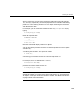

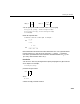
Table Of Contents
- Introduction
- LTI Models
- Operations on LTI Models
- Model Analysis Tools
- Arrays of LTI Models
- Customization
- Setting Toolbox Preferences
- Setting Tool Preferences
- Customizing Response Plot Properties
- Design Case Studies
- Reliable Computations
- GUI Reference
- SISO Design Tool Reference
- Menu Bar
- File
- Import
- Export
- Toolbox Preferences
- Print to Figure
- Close
- Edit
- Undo and Redo
- Root Locus and Bode Diagrams
- SISO Tool Preferences
- View
- Root Locus and Bode Diagrams
- System Data
- Closed Loop Poles
- Design History
- Tools
- Loop Responses
- Continuous/Discrete Conversions
- Draw a Simulink Diagram
- Compensator
- Format
- Edit
- Store
- Retrieve
- Clear
- Window
- Help
- Tool Bar
- Current Compensator
- Feedback Structure
- Root Locus Right-Click Menus
- Bode Diagram Right-Click Menus
- Status Panel
- Menu Bar
- LTI Viewer Reference
- Right-Click Menus for Response Plots
- Function Reference
- Functions by Category
- acker
- allmargin
- append
- augstate
- balreal
- bode
- bodemag
- c2d
- canon
- care
- chgunits
- connect
- covar
- ctrb
- ctrbf
- d2c
- d2d
- damp
- dare
- dcgain
- delay2z
- dlqr
- dlyap
- drss
- dsort
- dss
- dssdata
- esort
- estim
- evalfr
- feedback
- filt
- frd
- frdata
- freqresp
- gensig
- get
- gram
- hasdelay
- impulse
- initial
- interp
- inv
- isct, isdt
- isempty
- isproper
- issiso
- kalman
- kalmd
- lft
- lqgreg
- lqr
- lqrd
- lqry
- lsim
- ltimodels
- ltiprops
- ltiview
- lyap
- margin
- minreal
- modred
- ndims
- ngrid
- nichols
- norm
- nyquist
- obsv
- obsvf
- ord2
- pade
- parallel
- place
- pole
- pzmap
- reg
- reshape
- rlocus
- rss
- series
- set
- sgrid
- sigma
- sisotool
- size
- sminreal
- ss
- ss2ss
- ssbal
- ssdata
- stack
- step
- tf
- tfdata
- totaldelay
- zero
- zgrid
- zpk
- zpkdata
- Index

2 LTI Models
2-12
Zero-Pole-Gain Models
This section explains how to specify continuous-time SISO and MIMO
zero-pole-gain models. The specification for discrete-time zero-pole-gain
models is a simple extension of the continuous-time case. See “Discrete-Time
Models” on page 2-19.
SISO Zero-Pole-Gain Models
Continuous-time SISO zero-pole-gain models are of the form
where is a real-valued scalar (the gain), and ,..., and ,..., are the
real or complex conjugate pairs of zeros and poles of the transfer function .
This model is closely related to the transfer function representation: the zeros
are simply the numerator roots, and the poles, the denominator roots.
There are two ways to specify SISO zero-pole-gain models:
•Using the
zpk command
•As rational expressions in the Laplace variable s
ThesyntaxtospecifyZPKmodelsdirectlyusing
zpk is
h = zpk(z,p,k)
where z and p are the vectors of zeros and poles, and k is the gain. This
produces a ZPK object
h that encapsulates the z, p,andk data. For example,
typing
h = zpk(0, [1–i 1+i 2], –2)
produces
Zero/pole/gain:
–2 s
--------------------
(s–2) (s^2 – 2s + 2)
You can also specify zero-pole-gain models as rational expressions in the
Laplace variable s by:
hs
()
k
sz
1
–
()
... sz
m
–
()
sp
1
–
()
... sp
n
–
()
-------------------------------------------------
=
kz
1
z
m
p
1
p
n
hs
()