
Specifications
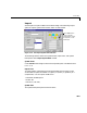
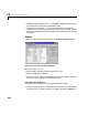
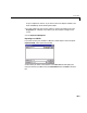
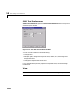
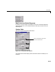
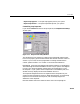

Table Of Contents
- Introduction
- LTI Models
- Operations on LTI Models
- Model Analysis Tools
- Arrays of LTI Models
- Customization
- Setting Toolbox Preferences
- Setting Tool Preferences
- Customizing Response Plot Properties
- Design Case Studies
- Reliable Computations
- GUI Reference
- SISO Design Tool Reference
- Menu Bar
- File
- Import
- Export
- Toolbox Preferences
- Print to Figure
- Close
- Edit
- Undo and Redo
- Root Locus and Bode Diagrams
- SISO Tool Preferences
- View
- Root Locus and Bode Diagrams
- System Data
- Closed Loop Poles
- Design History
- Tools
- Loop Responses
- Continuous/Discrete Conversions
- Draw a Simulink Diagram
- Compensator
- Format
- Edit
- Store
- Retrieve
- Clear
- Window
- Help
- Tool Bar
- Current Compensator
- Feedback Structure
- Root Locus Right-Click Menus
- Bode Diagram Right-Click Menus
- Status Panel
- Menu Bar
- LTI Viewer Reference
- Right-Click Menus for Response Plots
- Function Reference
- Functions by Category
- acker
- allmargin
- append
- augstate
- balreal
- bode
- bodemag
- c2d
- canon
- care
- chgunits
- connect
- covar
- ctrb
- ctrbf
- d2c
- d2d
- damp
- dare
- dcgain
- delay2z
- dlqr
- dlyap
- drss
- dsort
- dss
- dssdata
- esort
- estim
- evalfr
- feedback
- filt
- frd
- frdata
- freqresp
- gensig
- get
- gram
- hasdelay
- impulse
- initial
- interp
- inv
- isct, isdt
- isempty
- isproper
- issiso
- kalman
- kalmd
- lft
- lqgreg
- lqr
- lqrd
- lqry
- lsim
- ltimodels
- ltiprops
- ltiview
- lyap
- margin
- minreal
- modred
- ndims
- ngrid
- nichols
- norm
- nyquist
- obsv
- obsvf
- ord2
- pade
- parallel
- place
- pole
- pzmap
- reg
- reshape
- rlocus
- rss
- series
- set
- sgrid
- sigma
- sisotool
- size
- sminreal
- ss
- ss2ss
- ssbal
- ssdata
- stack
- step
- tf
- tfdata
- totaldelay
- zero
- zgrid
- zpk
- zpkdata
- Index

13 SISO Design Tool Reference
13-14
•Loop transfer — This is defined as the compensator (C), the plant (G), and
the sensor (
H) multiplied together (CGH). If you haven’tdefinedasensor,its
default value is 1.
•Sensitivity function — This is defined as , where L is the loop transfer
function.
Some of the open- and closed-loop responses use these definitions. See
“Contents of plots” for more information.
Plots. You can have up to six plots in one LTI Viewer. By default, the Response
Plot Setup window specifies one step response plot. To reconfigure the LTI
Viewer for more plots, start by selecting “2. None” from the list of plots and
thenspecifyanewplottypein the
Changeto field. Plot types available include
the following:
•Step
•Impulse
•Bode
•Bode Magnitude
•Nyquist
•Nichols
•Sigma
•Pzmap (pole/zero map)
•None (deselect a plot)
Note that you do not have to select adjacent numbers; for example, if you
specifyplot#1tobeastepresponse,plot#2tobenone,andplot#3tobean
impulse response, the LTI Viewer will open with two plots, a step and an
impulse response. There will not be an empty plot region.
Contents of plots. Once you have selected a plot, you can specify various open-
andclosed-looptransfer functions.Youcan plot open-loop responses foreachof
the components of your system, including your compensator (
C), plant (G),
prefilter (
F), or sensor (H). In addition, loop transfer and sensitivity transfer
functions are available. Their definitions are listed in the Response Plot Setup
window.
See the block diagram in Figure 13-7, Response Plot Setup Window for
definitions of the input/output points for closed-loop responses.
1
1 L+
-------------