
Specifications
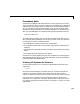
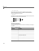

Table Of Contents
- Introduction
- LTI Models
- Operations on LTI Models
- Model Analysis Tools
- Arrays of LTI Models
- Customization
- Setting Toolbox Preferences
- Setting Tool Preferences
- Customizing Response Plot Properties
- Design Case Studies
- Reliable Computations
- GUI Reference
- SISO Design Tool Reference
- Menu Bar
- File
- Import
- Export
- Toolbox Preferences
- Print to Figure
- Close
- Edit
- Undo and Redo
- Root Locus and Bode Diagrams
- SISO Tool Preferences
- View
- Root Locus and Bode Diagrams
- System Data
- Closed Loop Poles
- Design History
- Tools
- Loop Responses
- Continuous/Discrete Conversions
- Draw a Simulink Diagram
- Compensator
- Format
- Edit
- Store
- Retrieve
- Clear
- Window
- Help
- Tool Bar
- Current Compensator
- Feedback Structure
- Root Locus Right-Click Menus
- Bode Diagram Right-Click Menus
- Status Panel
- Menu Bar
- LTI Viewer Reference
- Right-Click Menus for Response Plots
- Function Reference
- Functions by Category
- acker
- allmargin
- append
- augstate
- balreal
- bode
- bodemag
- c2d
- canon
- care
- chgunits
- connect
- covar
- ctrb
- ctrbf
- d2c
- d2d
- damp
- dare
- dcgain
- delay2z
- dlqr
- dlyap
- drss
- dsort
- dss
- dssdata
- esort
- estim
- evalfr
- feedback
- filt
- frd
- frdata
- freqresp
- gensig
- get
- gram
- hasdelay
- impulse
- initial
- interp
- inv
- isct, isdt
- isempty
- isproper
- issiso
- kalman
- kalmd
- lft
- lqgreg
- lqr
- lqrd
- lqry
- lsim
- ltimodels
- ltiprops
- ltiview
- lyap
- margin
- minreal
- modred
- ndims
- ngrid
- nichols
- norm
- nyquist
- obsv
- obsvf
- ord2
- pade
- parallel
- place
- pole
- pzmap
- reg
- reshape
- rlocus
- rss
- series
- set
- sgrid
- sigma
- sisotool
- size
- sminreal
- ss
- ss2ss
- ssbal
- ssdata
- stack
- step
- tf
- tfdata
- totaldelay
- zero
- zgrid
- zpk
- zpkdata
- Index

2 LTI Models
2-10
MIMO Transfer Function Models
MIMO transfer functions are two-dimensional arrays of elementary SISO
transfer functions. There are several ways to specify MIMO transfer function
models, including:
•Concatenation of SISO transfer function models
•Using
tf with cell array arguments
Consider the rational transfer matrix
.
You can specify by concatenation of its SISO entries. For instance,
h11 = tf([1 –1],[1 1]);
h21 = tf([1 2],[1 4 5]);
or, equivalently,
s = tf('s')
h11 = (s–1)/(s+1);
h21 = (s+2)/(s^2+4*s+5);
can be concatenated to form .
H = [h11; h21]
This syntax mimics standard matrix concatenation and tends to be easier and
morereadable forMIMOsystemswithmanyinputsand/oroutputs.See“Model
Interconnection Functions” on page 3-16 for more details on concatenation
operations for LTI systems.
Alternatively, to define MIMO transfer functions using
tf, you need two cell
arrays (say,
N and D) to represent the sets of numerator and denominator
polynomials, respectively. See Chapter 13, “Structures and Cell Arrays” in
Using MATLAB for more details on cell arrays.
For example, for the rational transfer matrix , the two cell arrays
N and D
should contain the row-vector representations of the polynomial entries of
Hs
()
s 1–
s 1+
------------
s 2+
s
2
4s 5++
----------------------------
=
Hs
(
)
Hs
()
Hs()